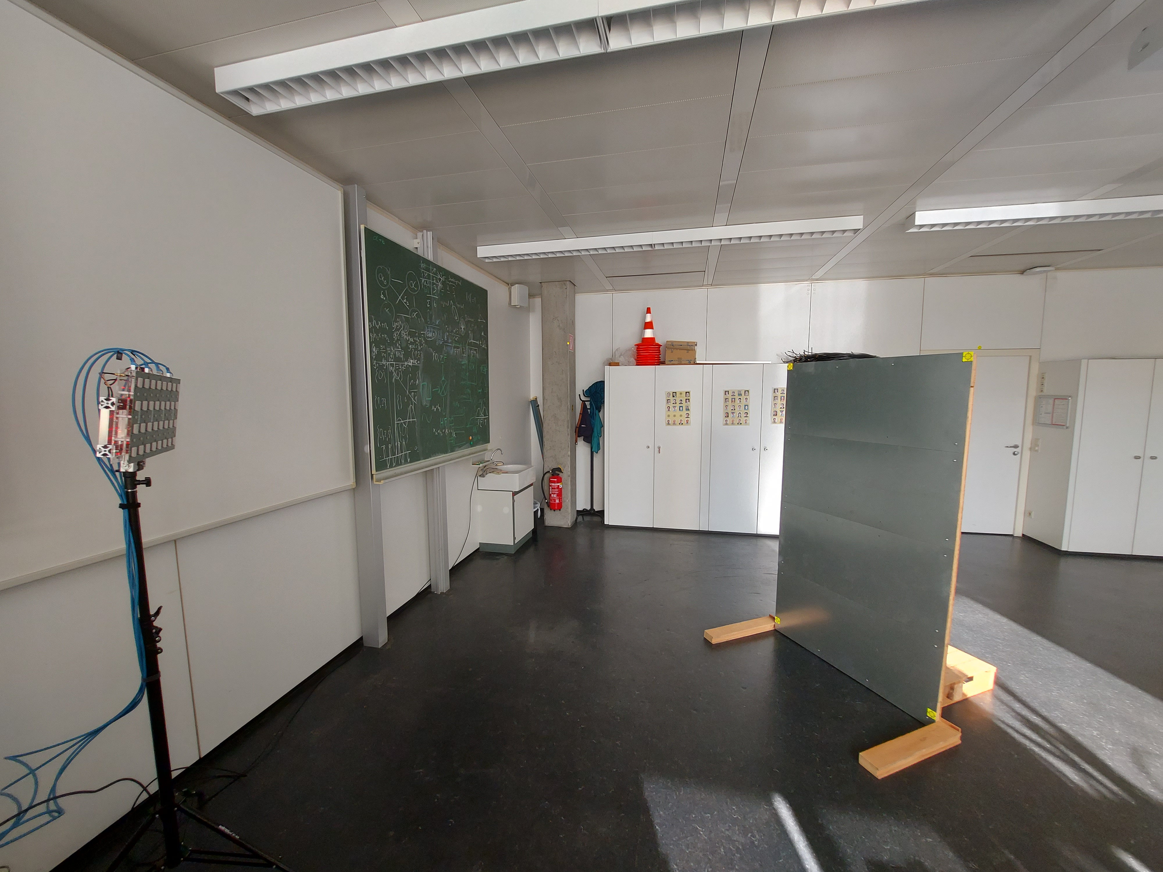
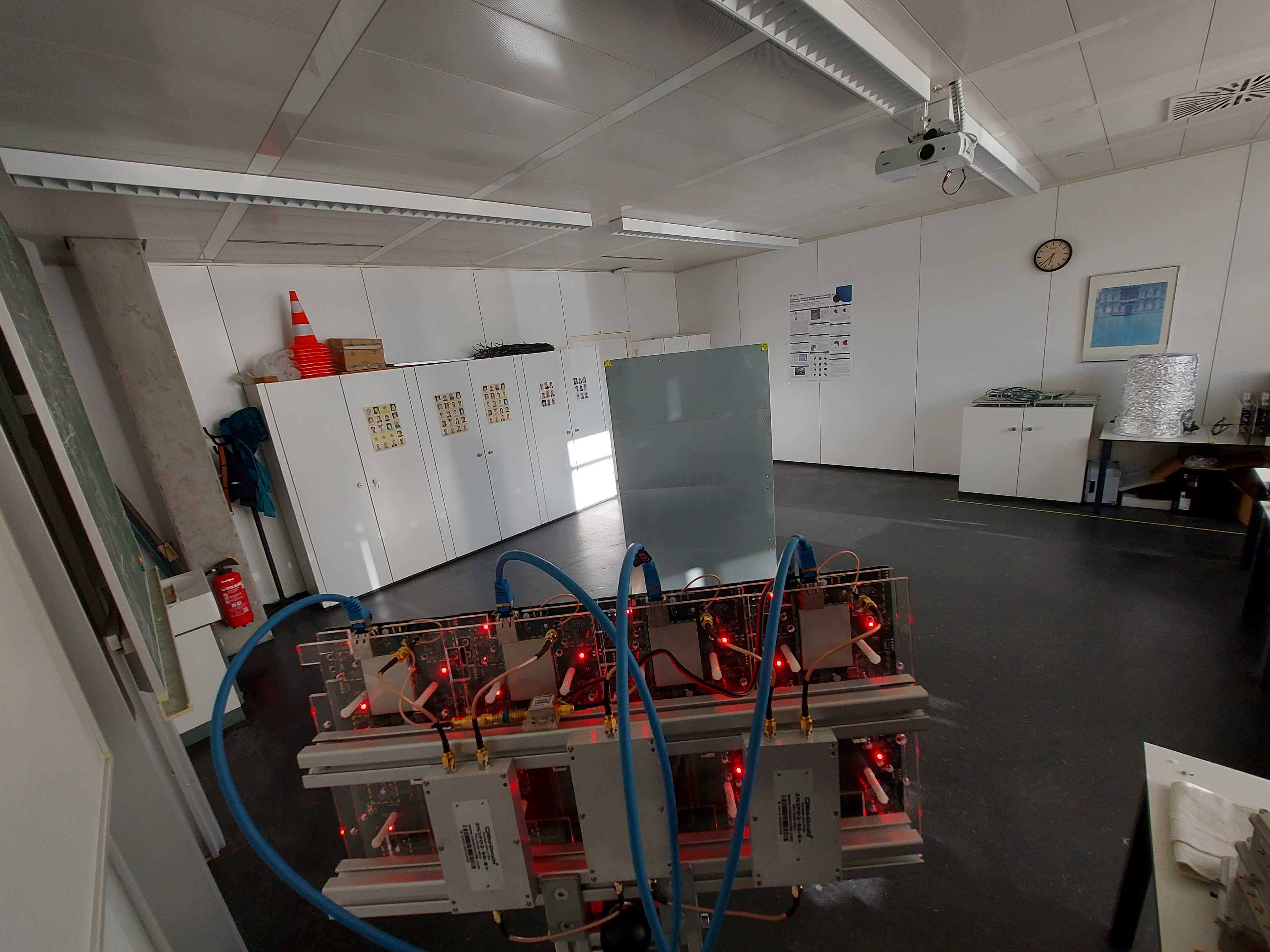
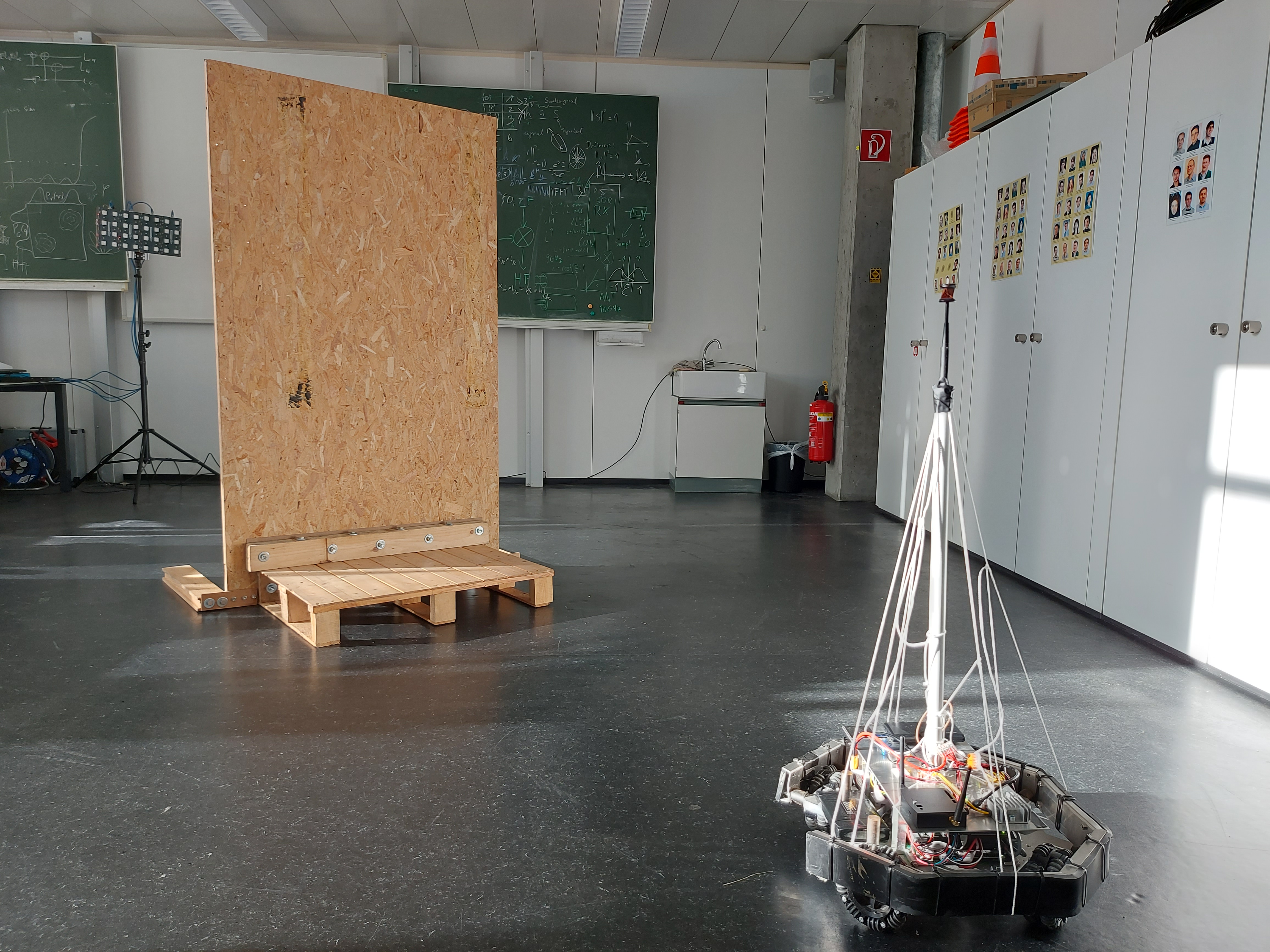
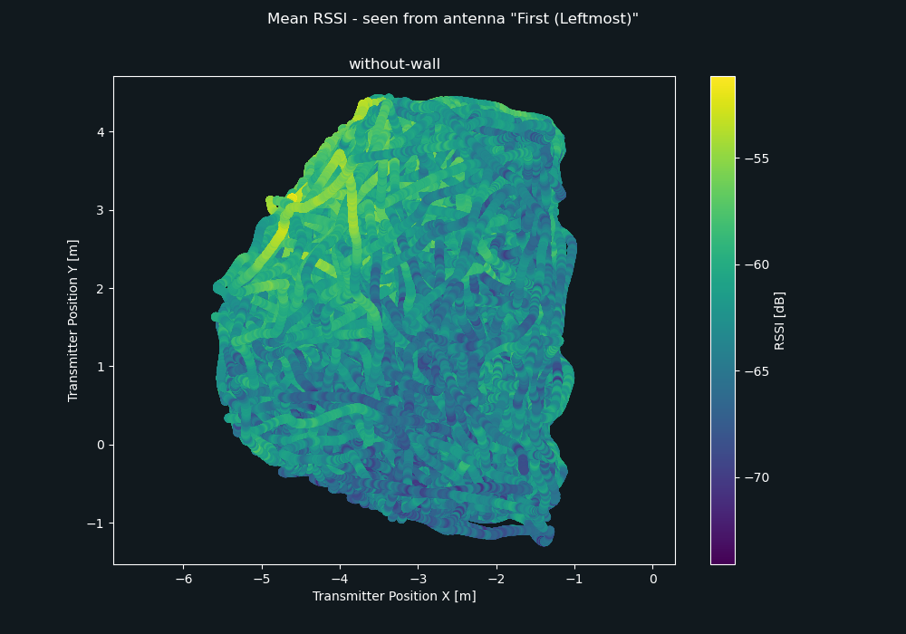
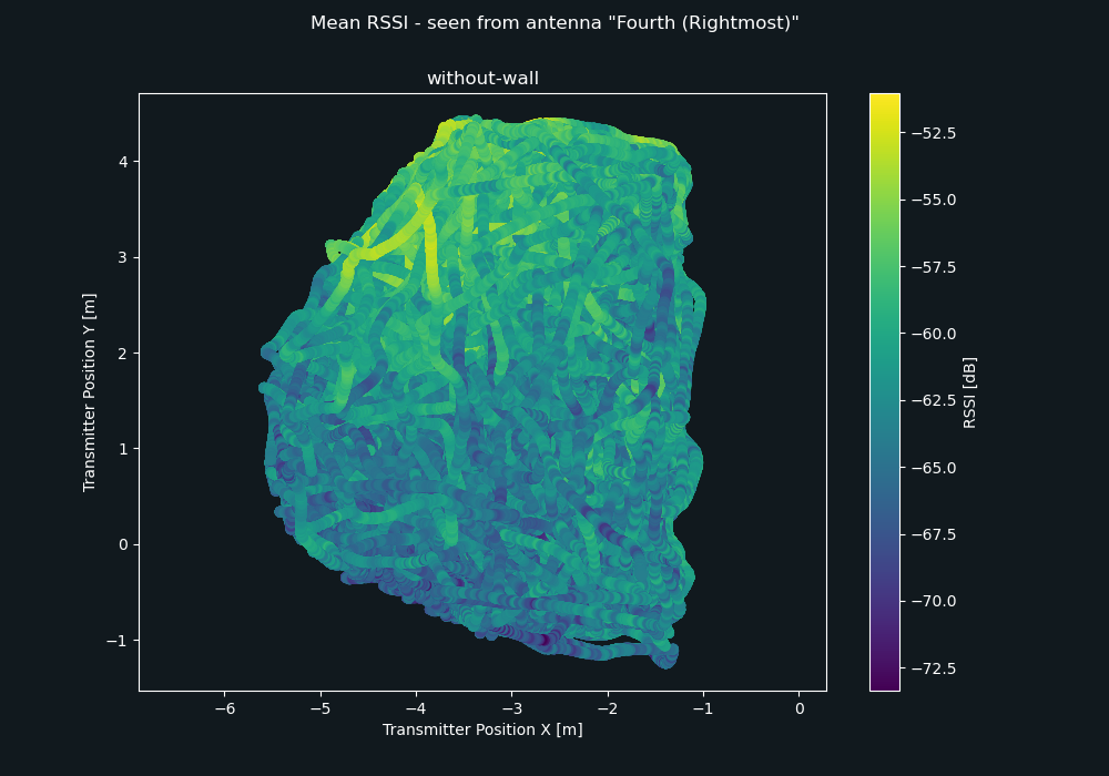
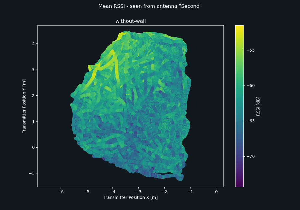
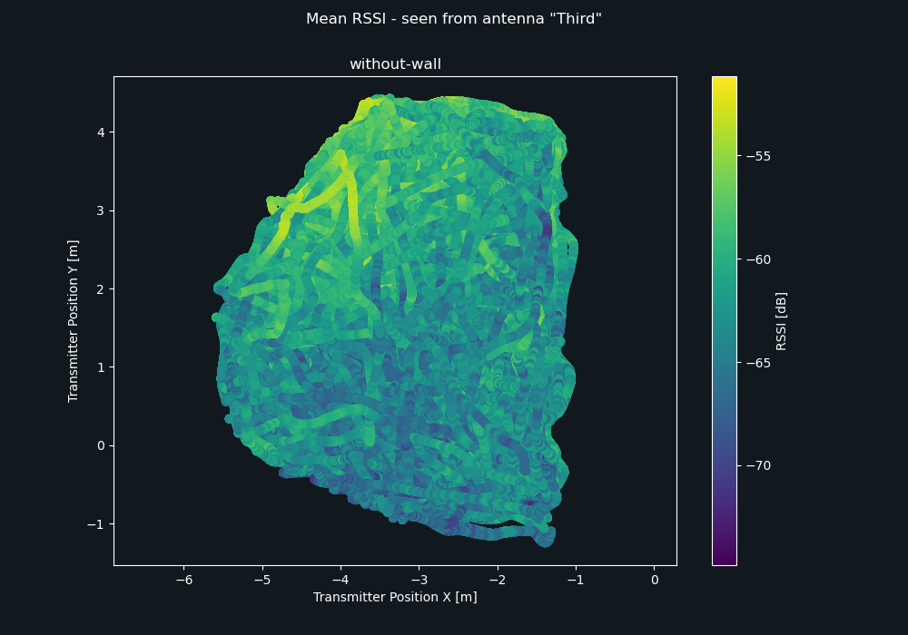
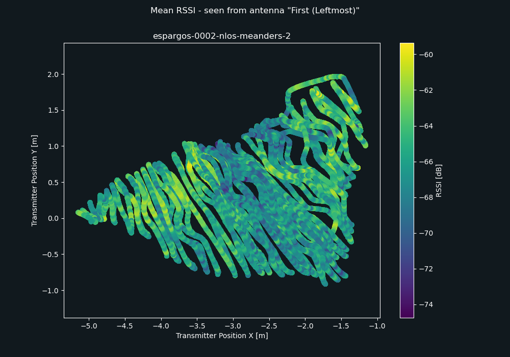
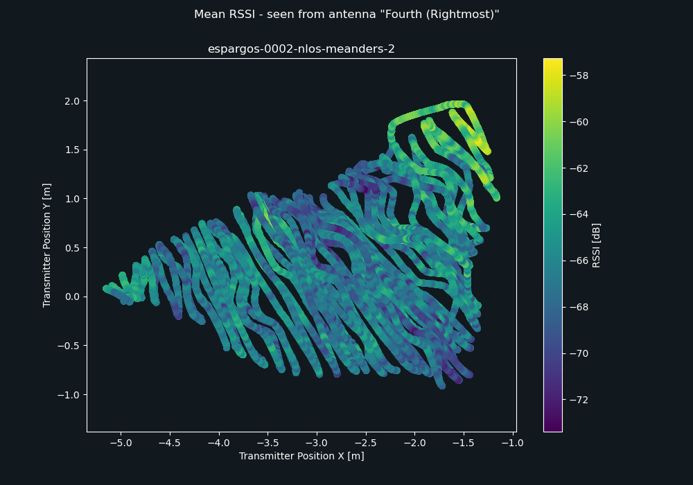
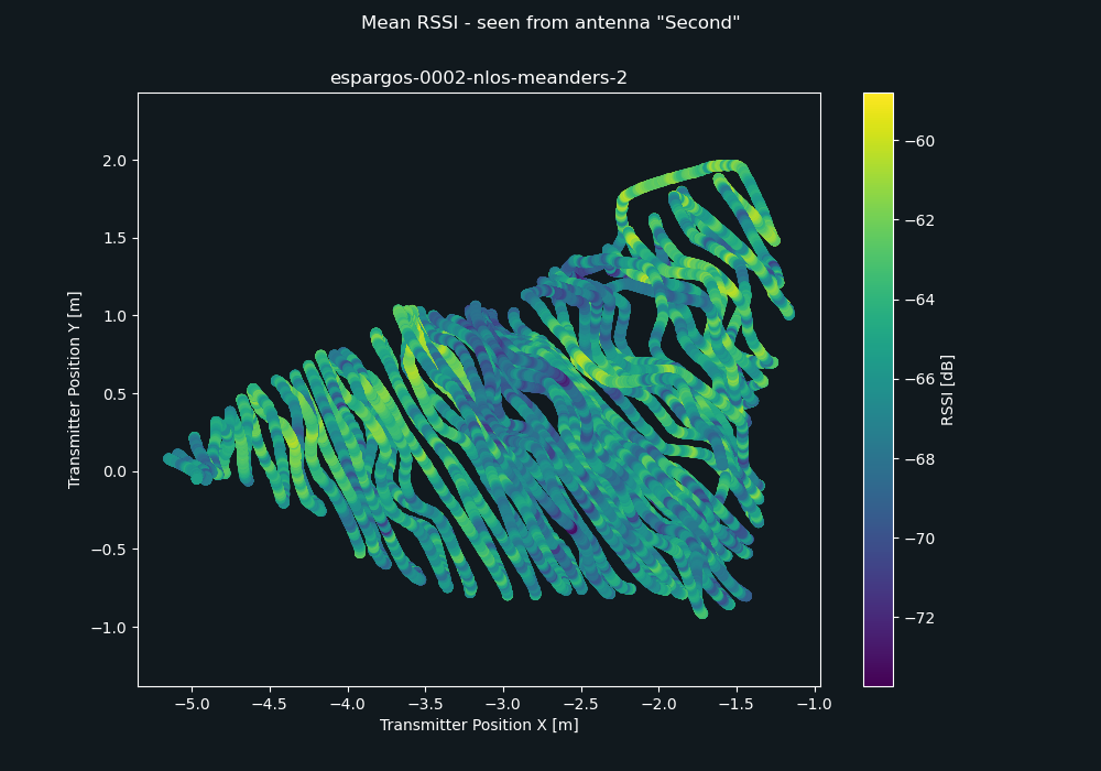
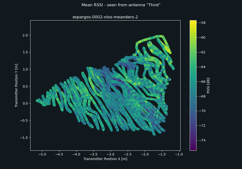
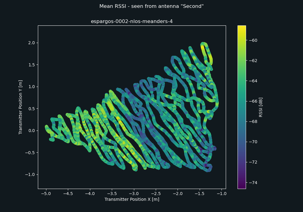
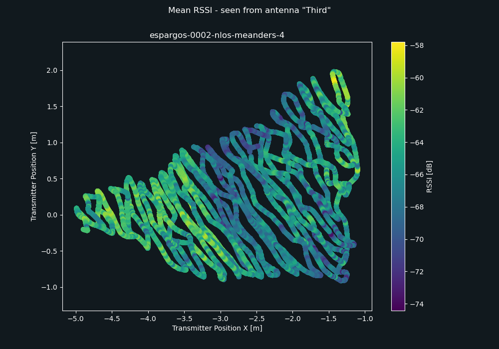
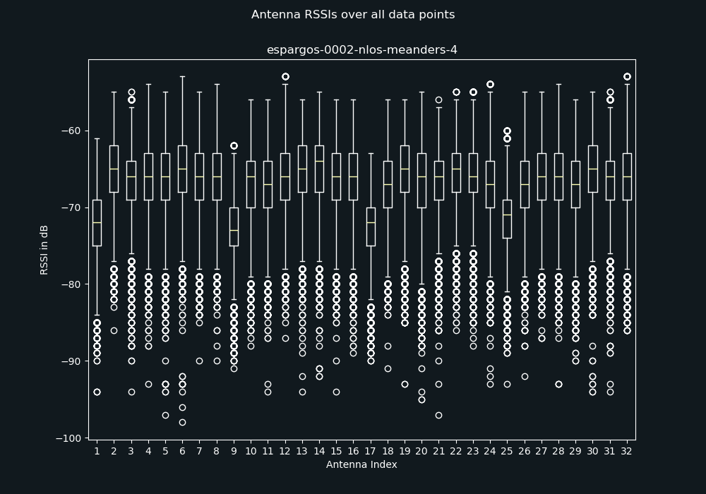
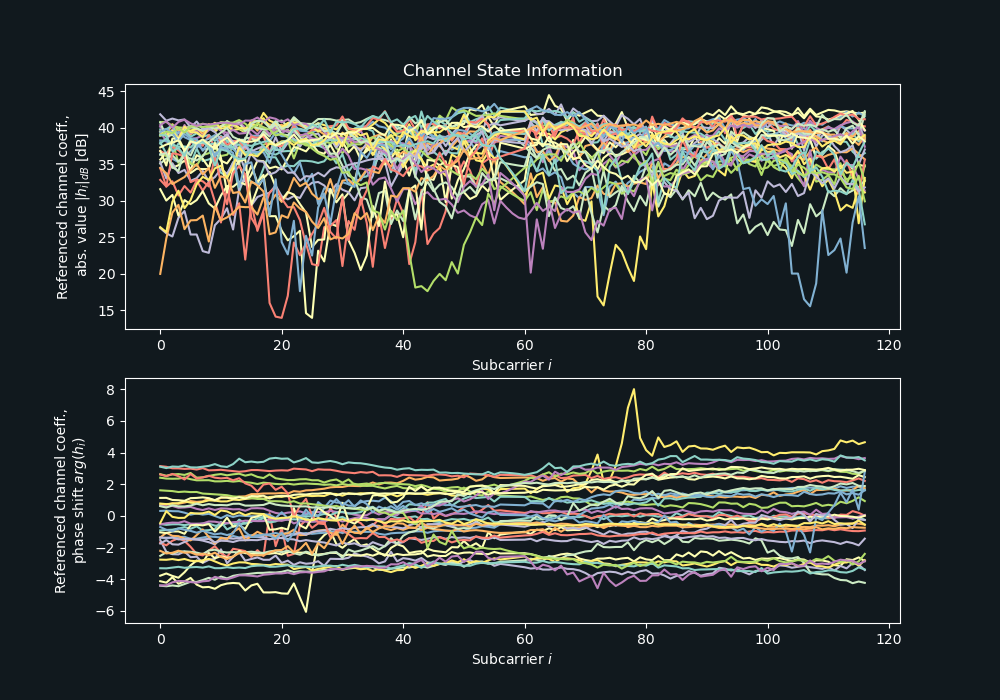
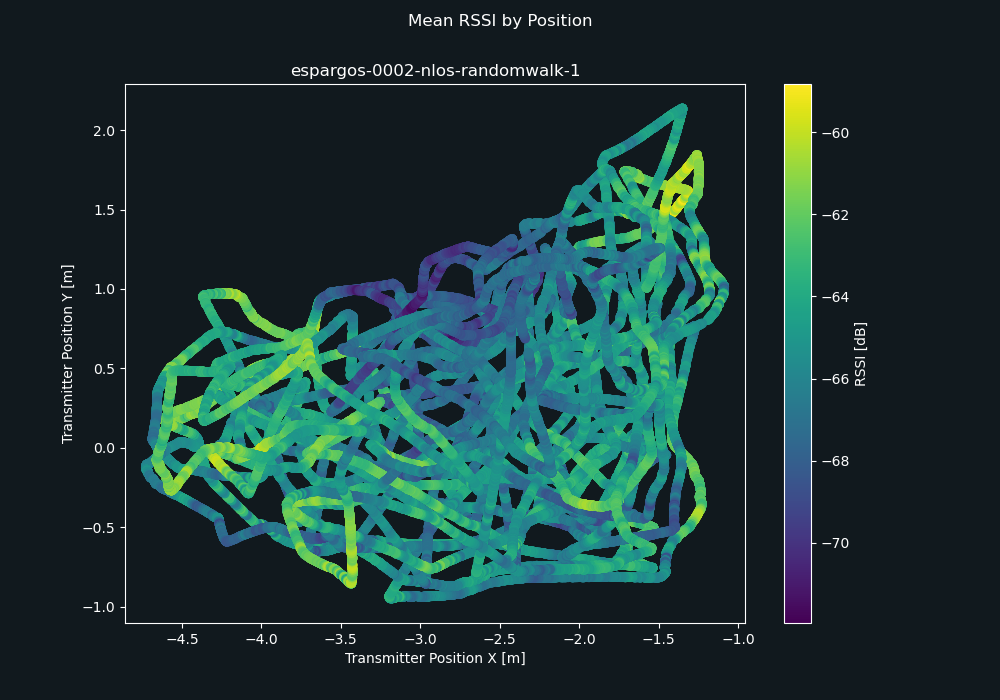
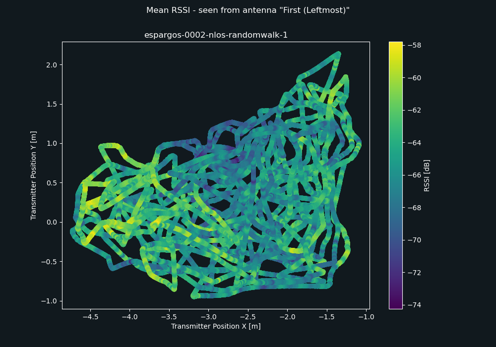
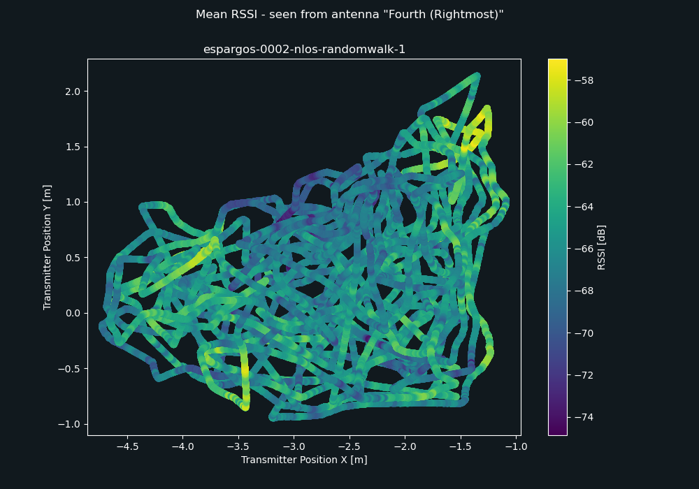
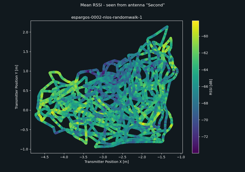
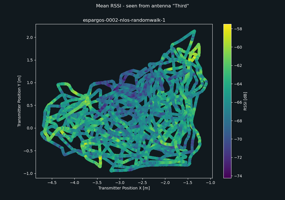
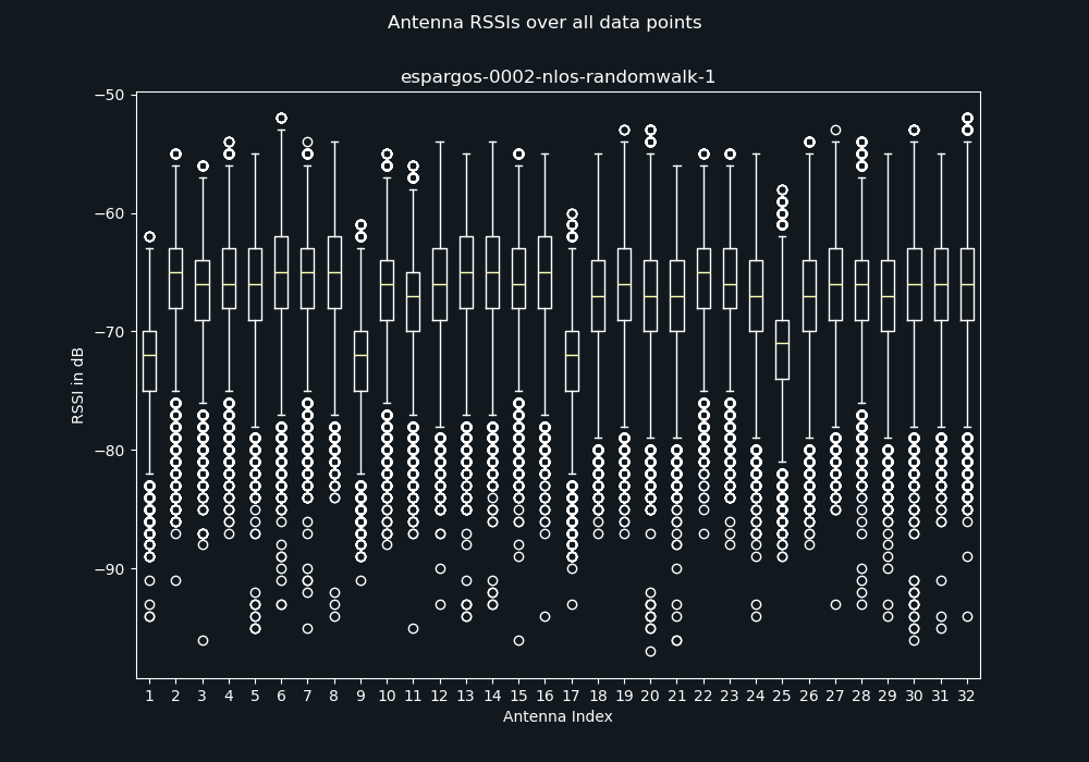
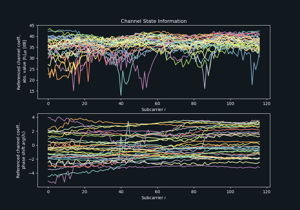
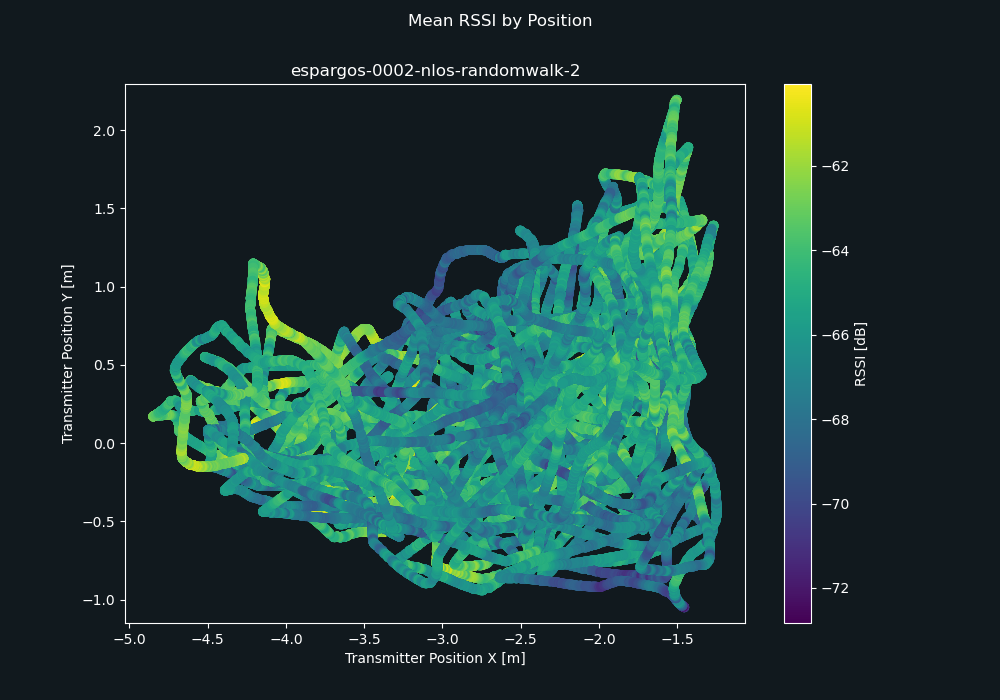
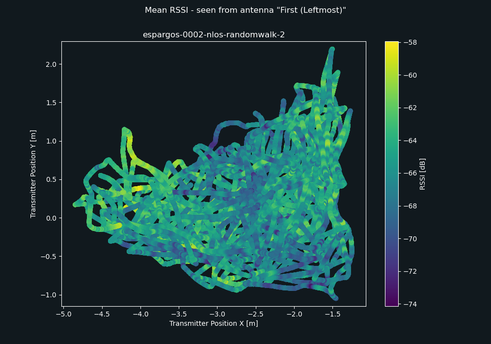
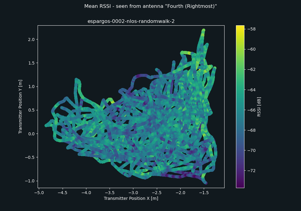
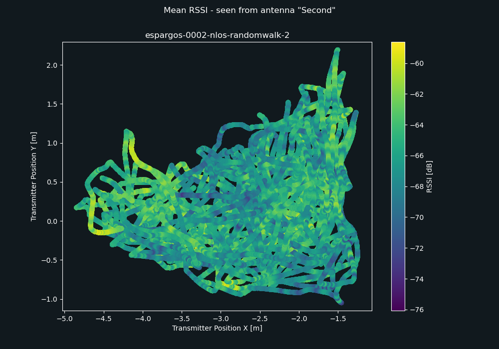
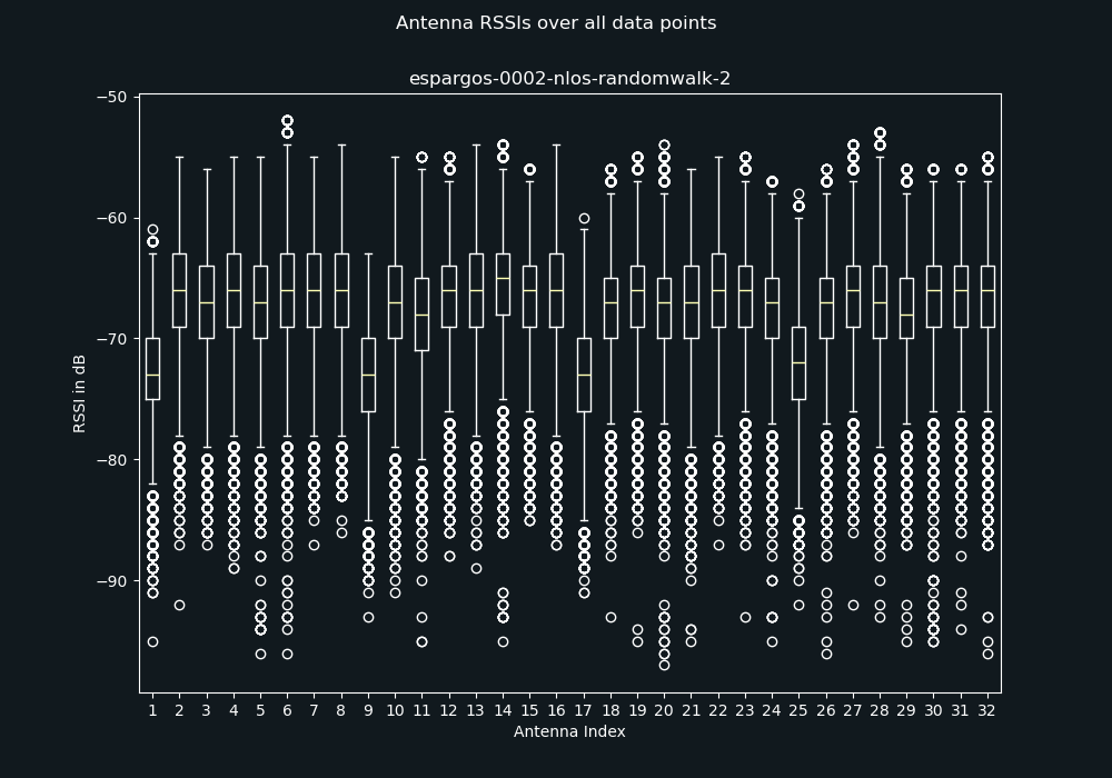
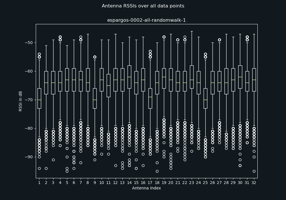
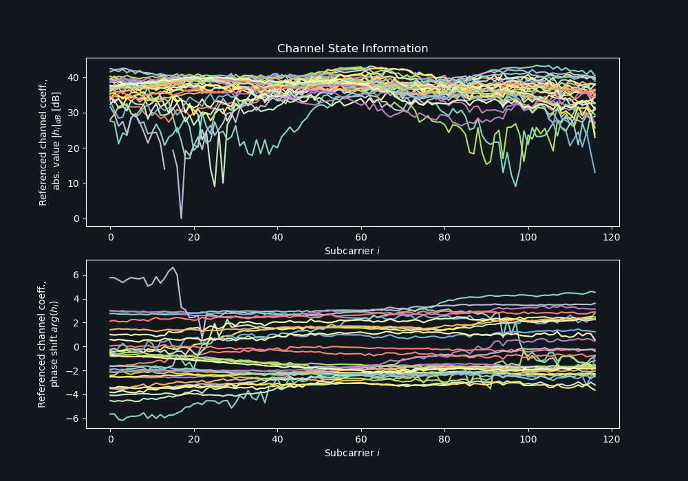
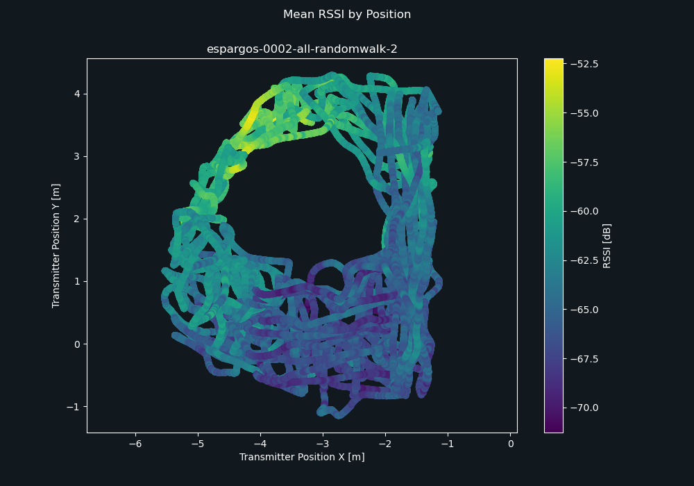
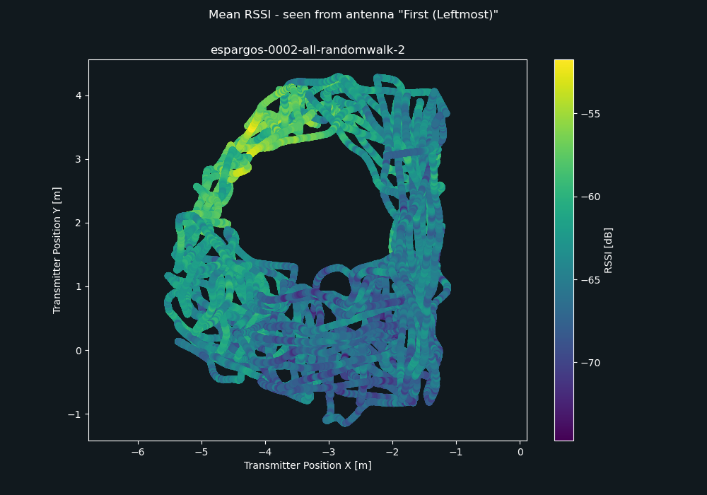
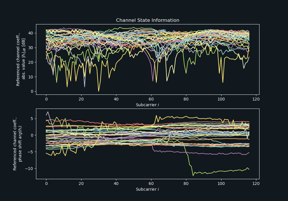
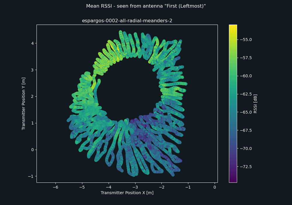
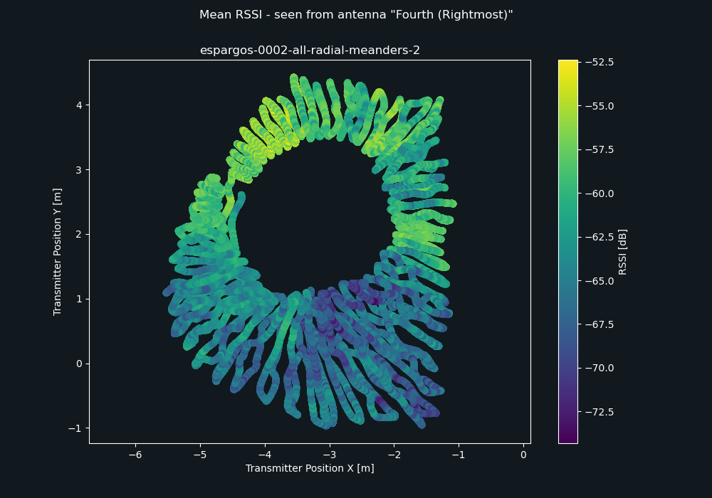
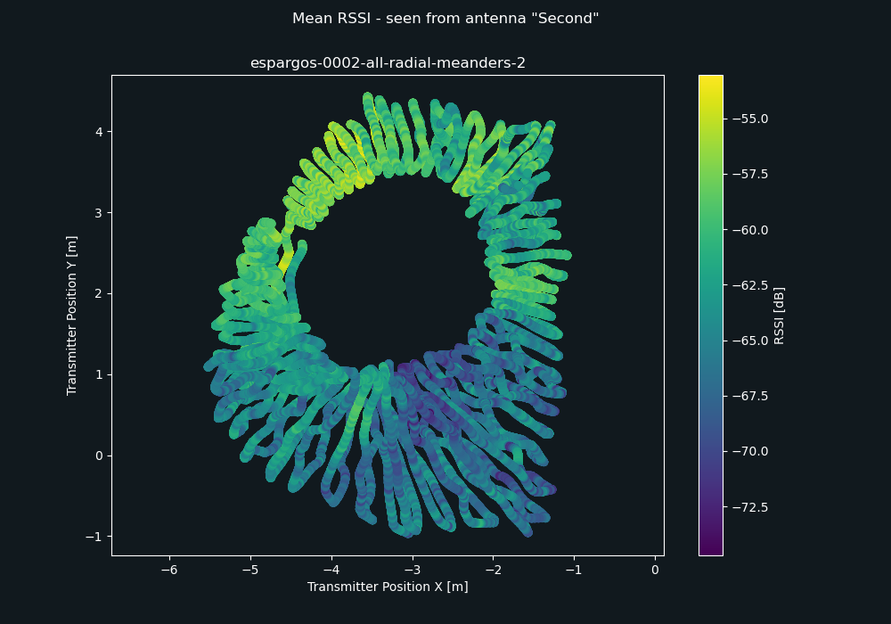
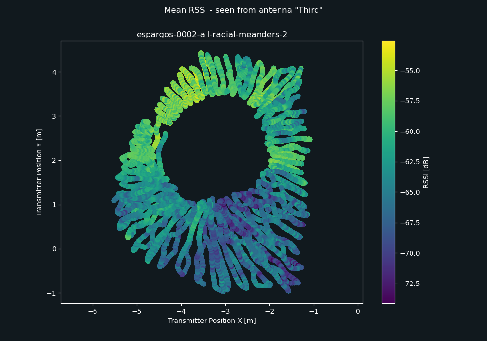
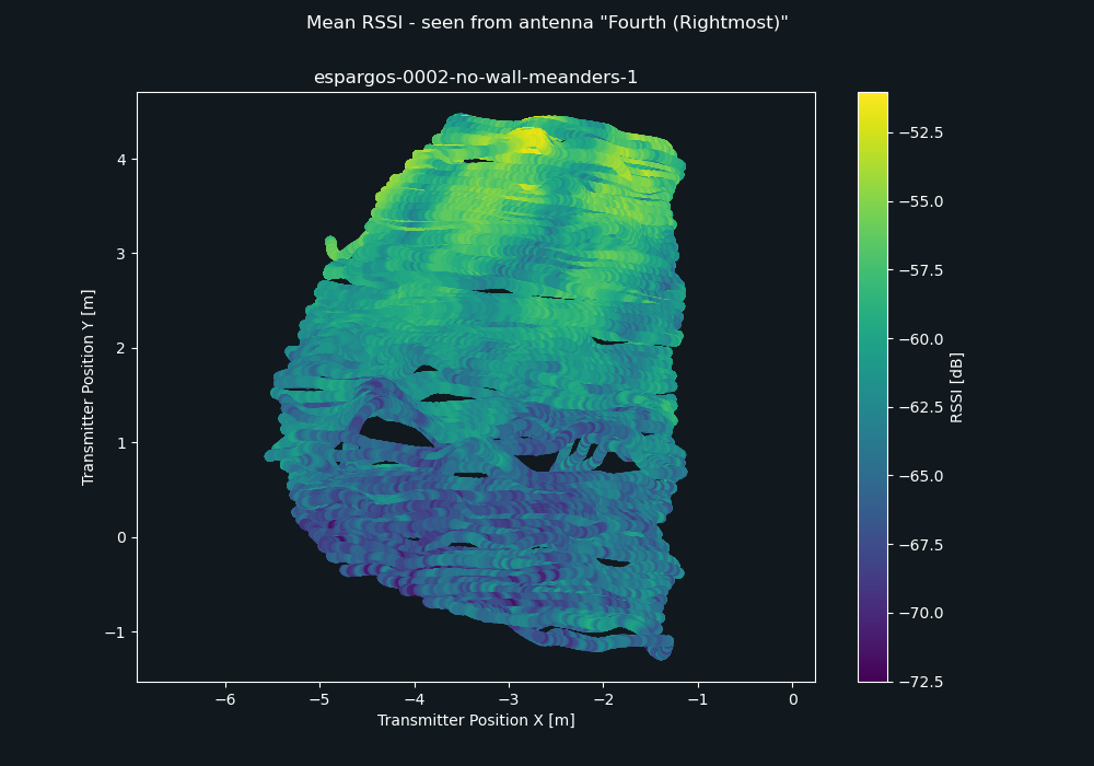
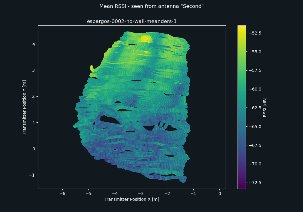
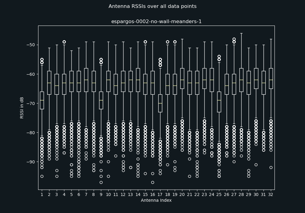
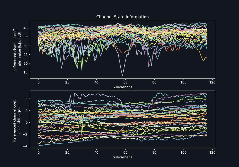
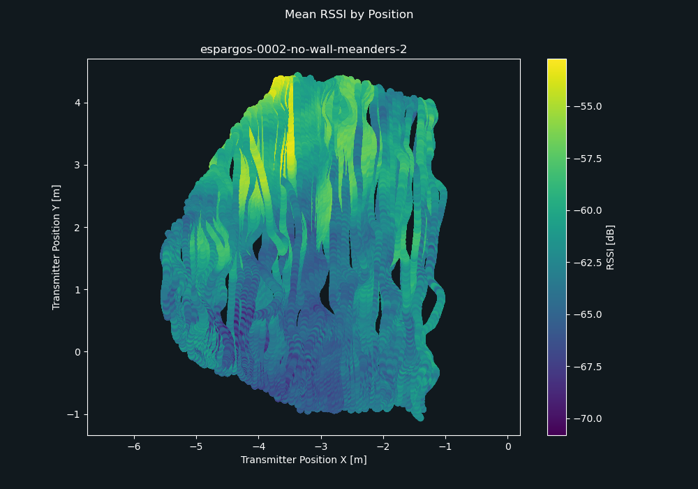
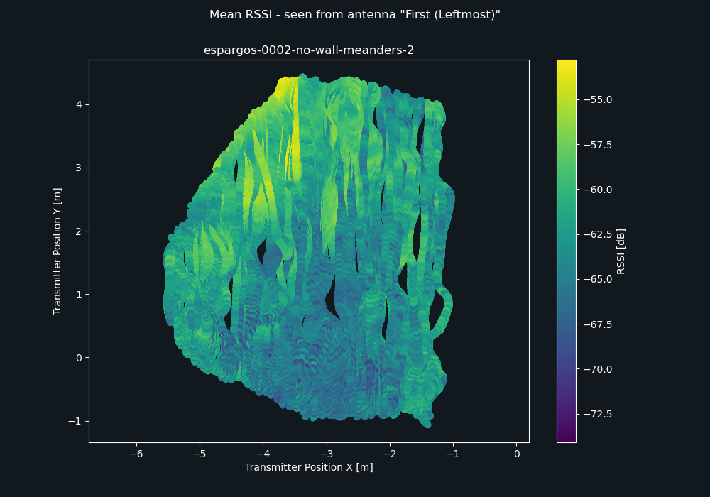
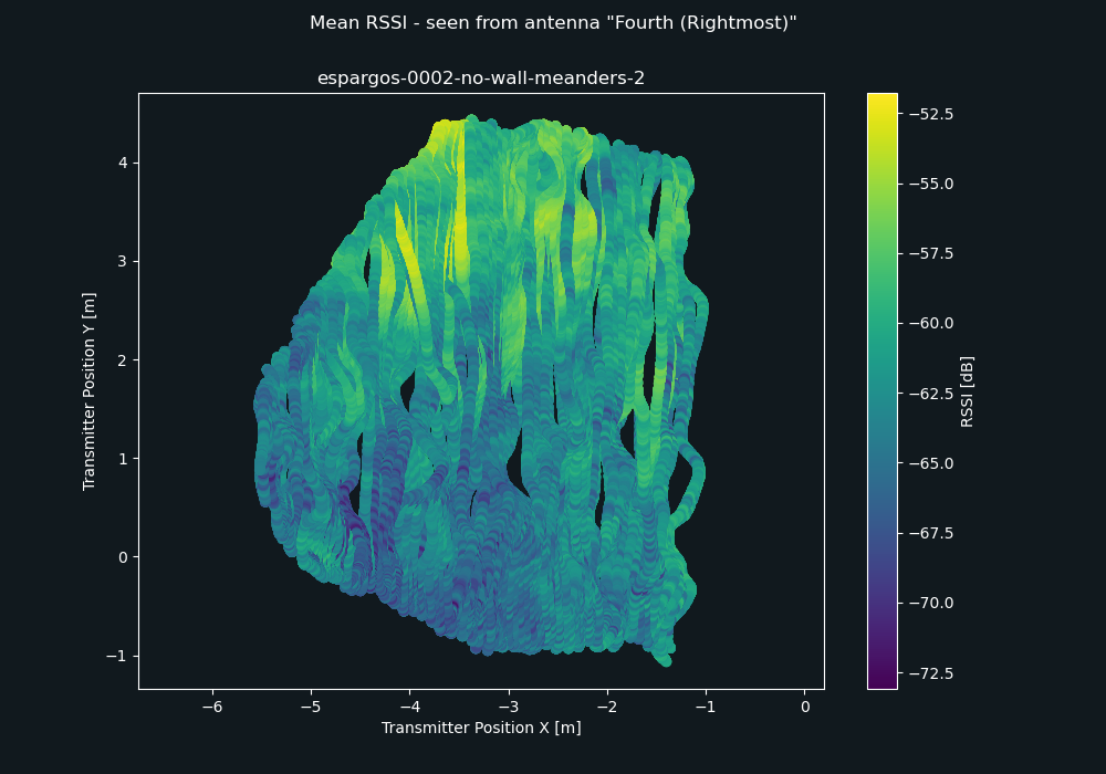
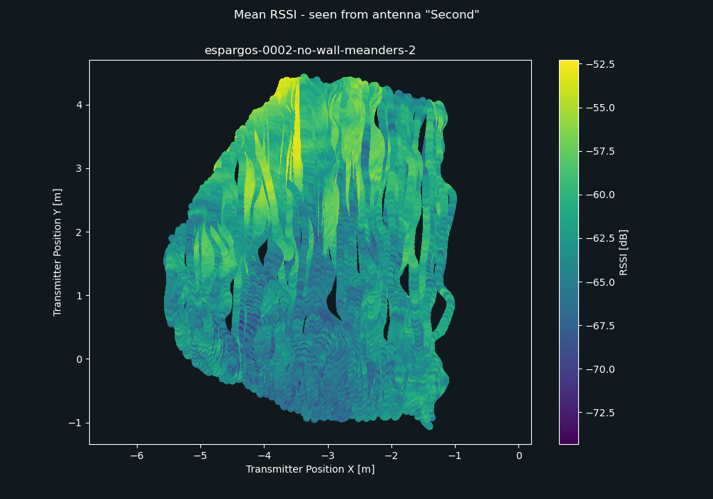
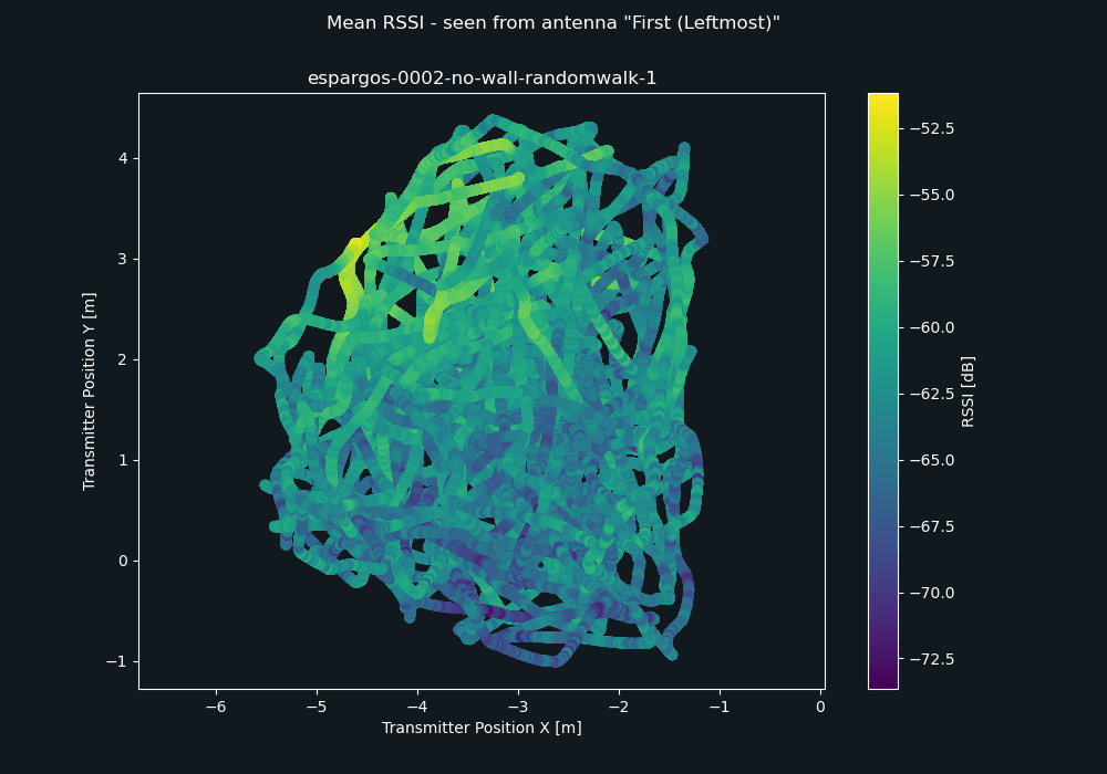
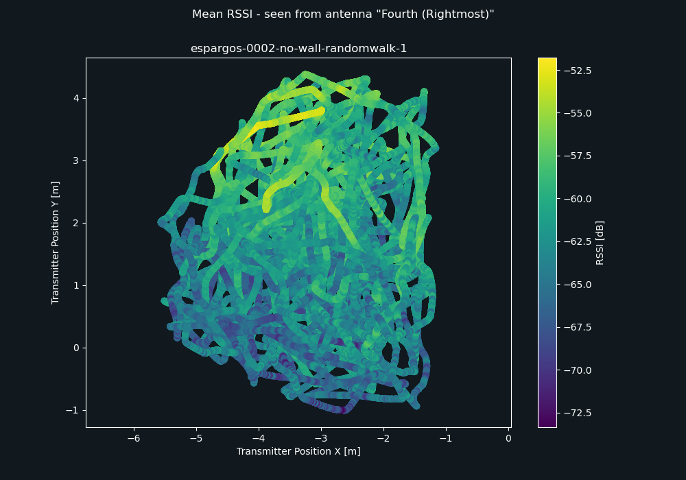
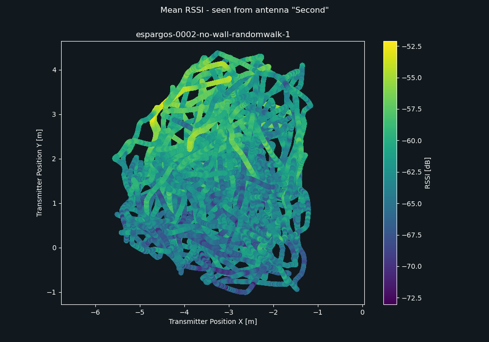
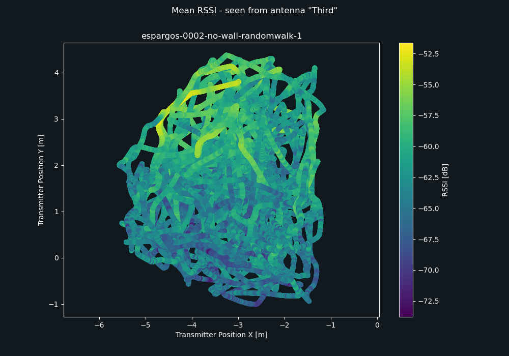
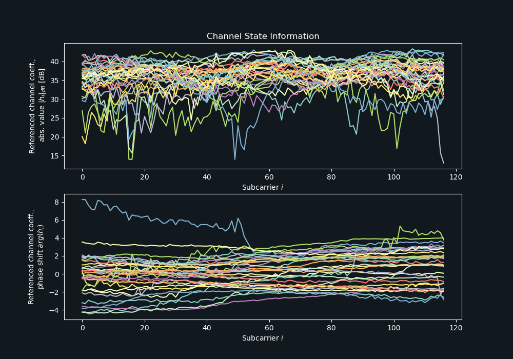
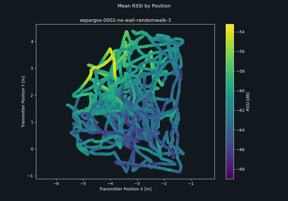
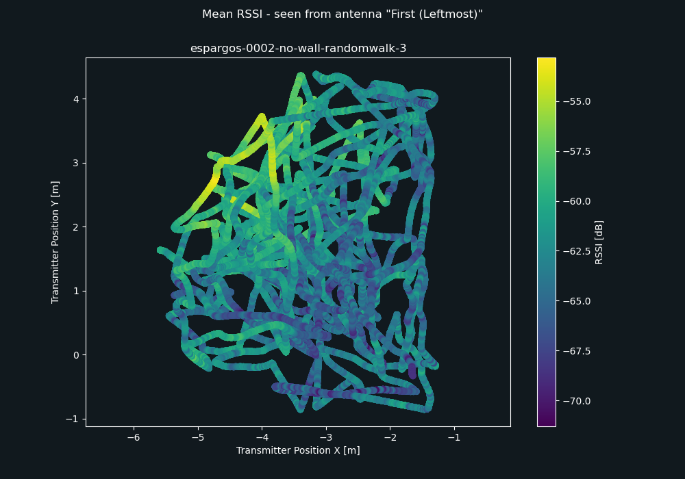
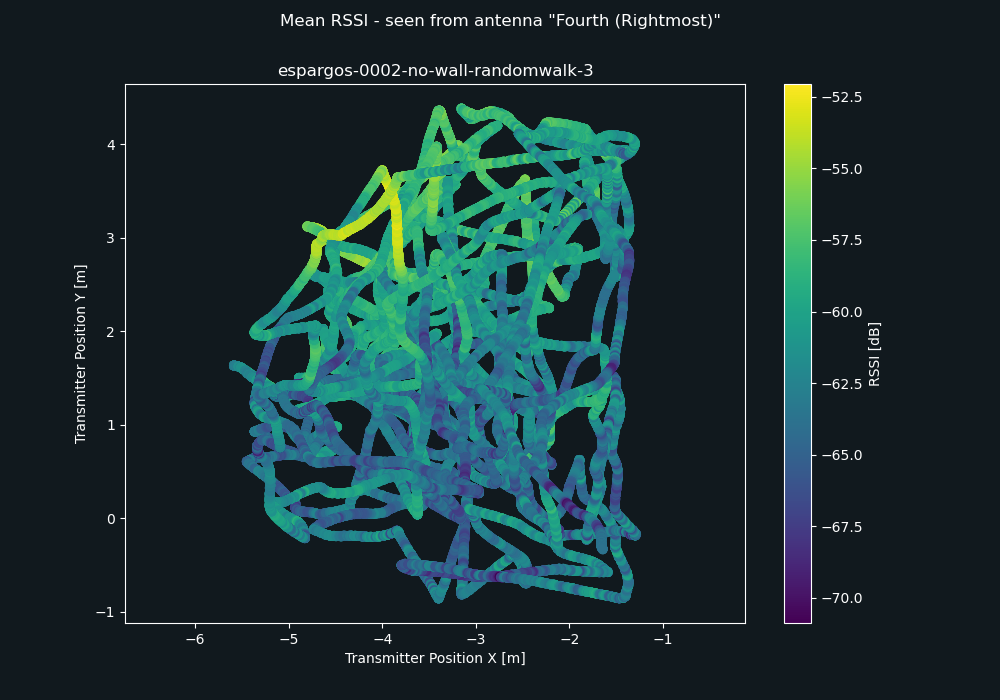
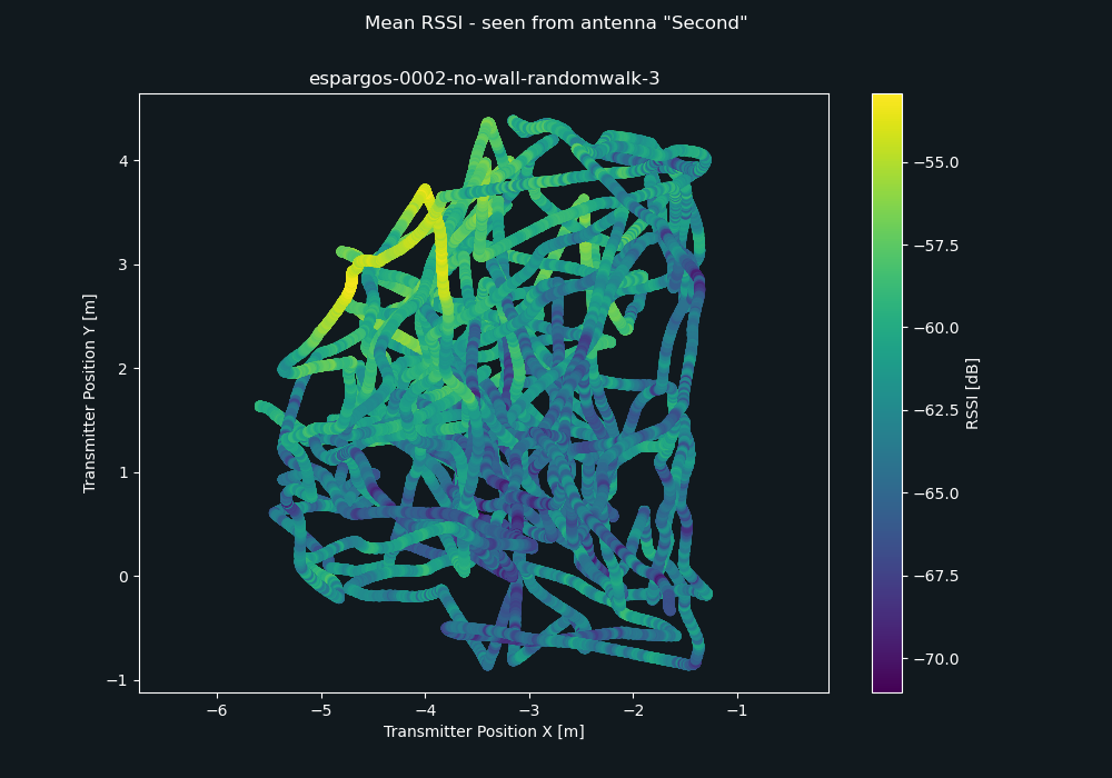
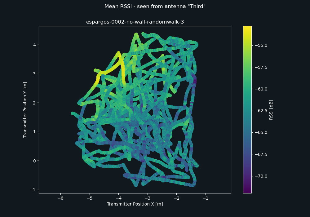
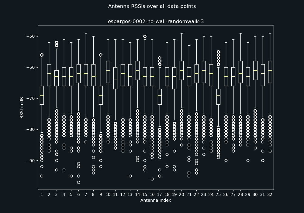
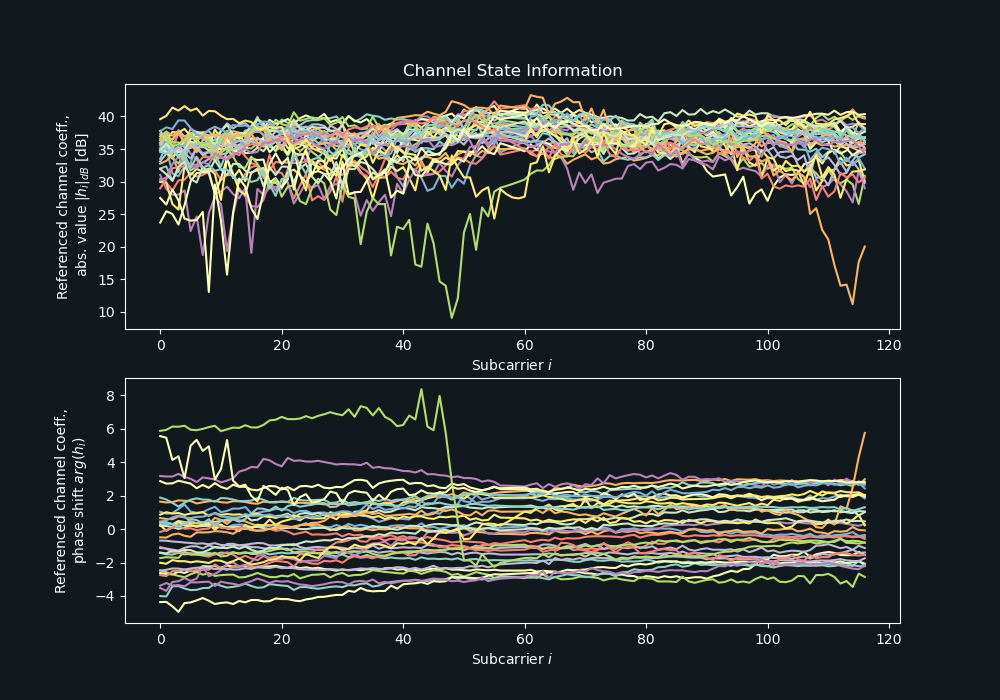
espargos-0002 Dataset: Larger combined antenna array, indoor lab room with metal wall, LoS and NLoS areas
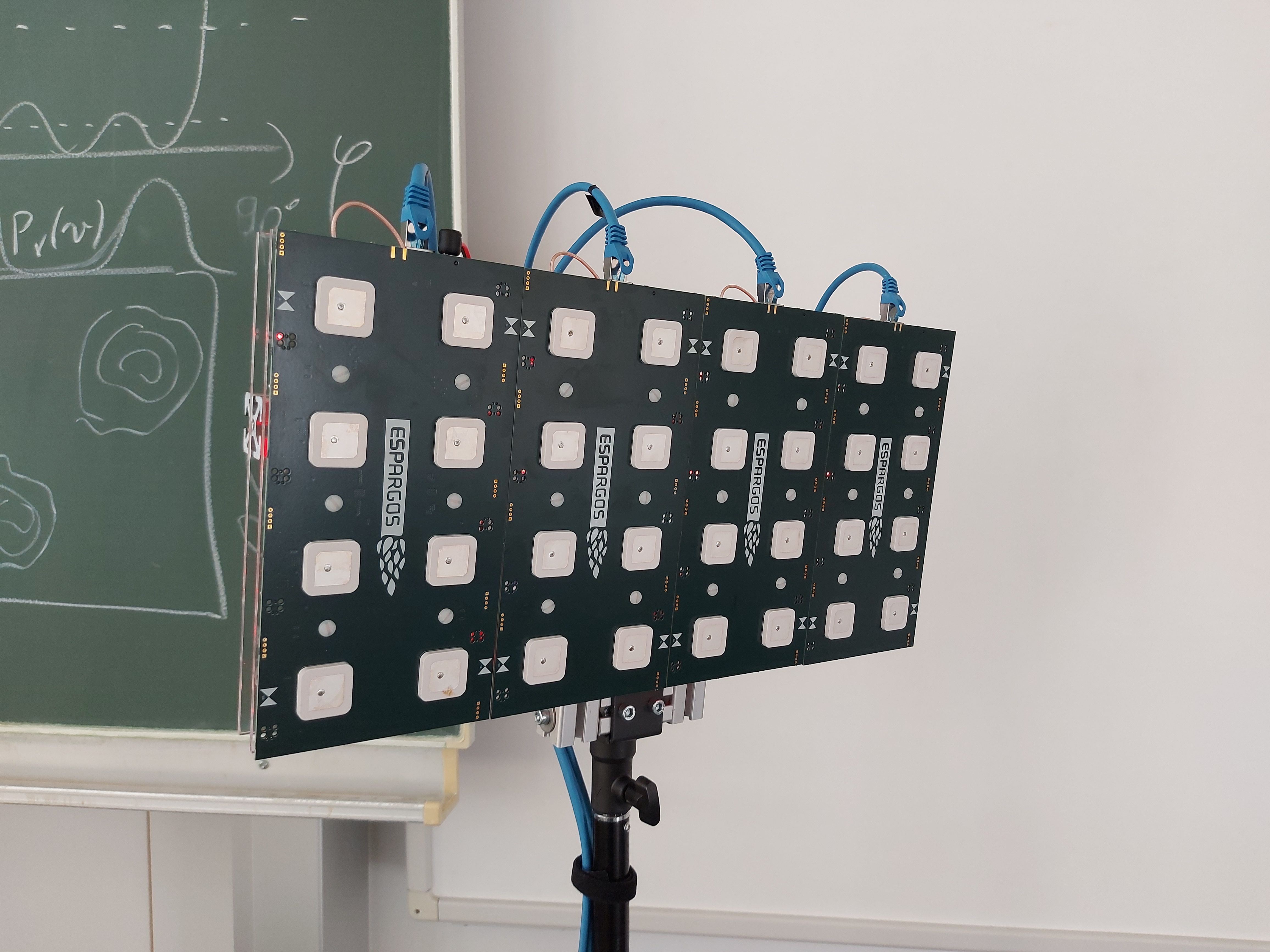
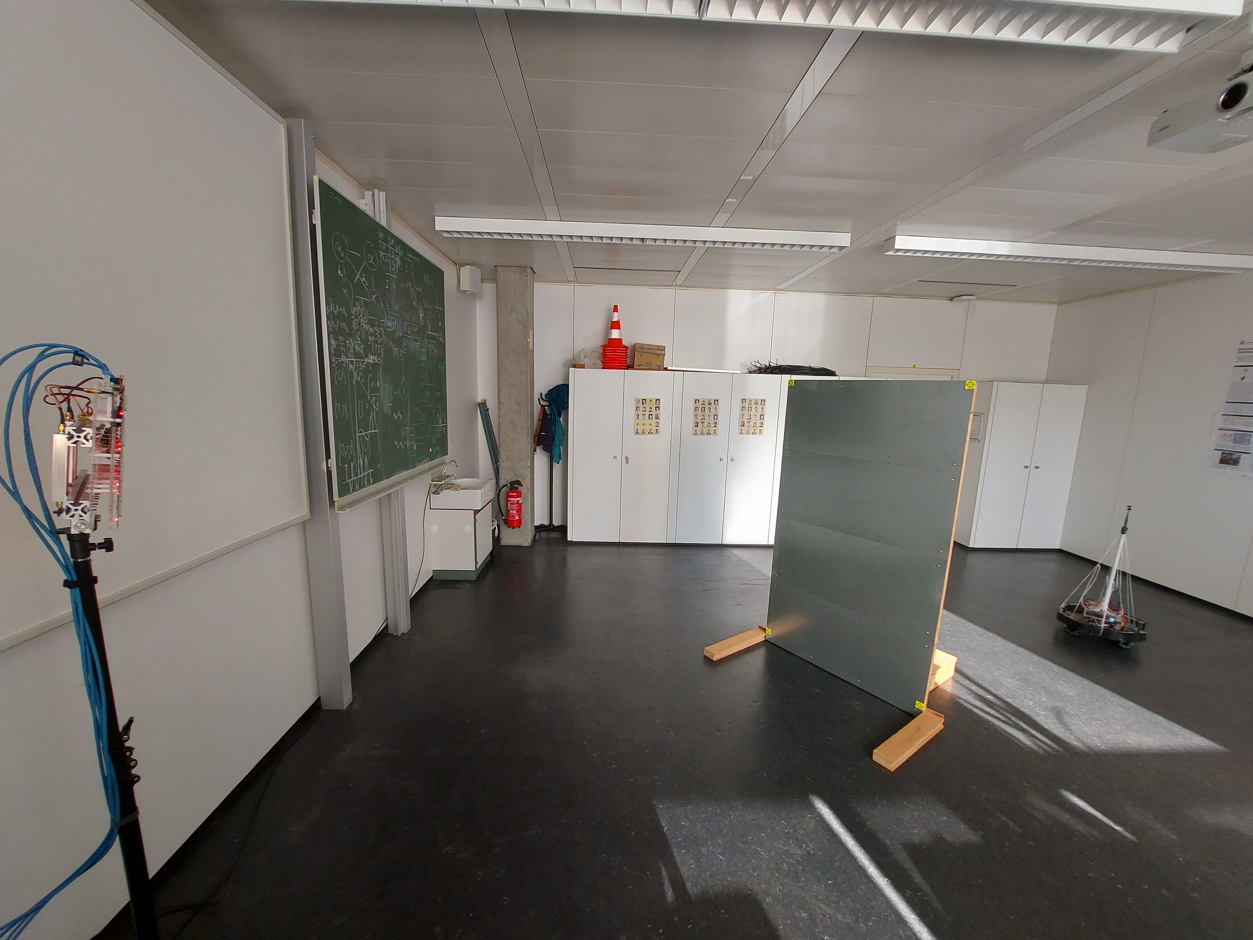
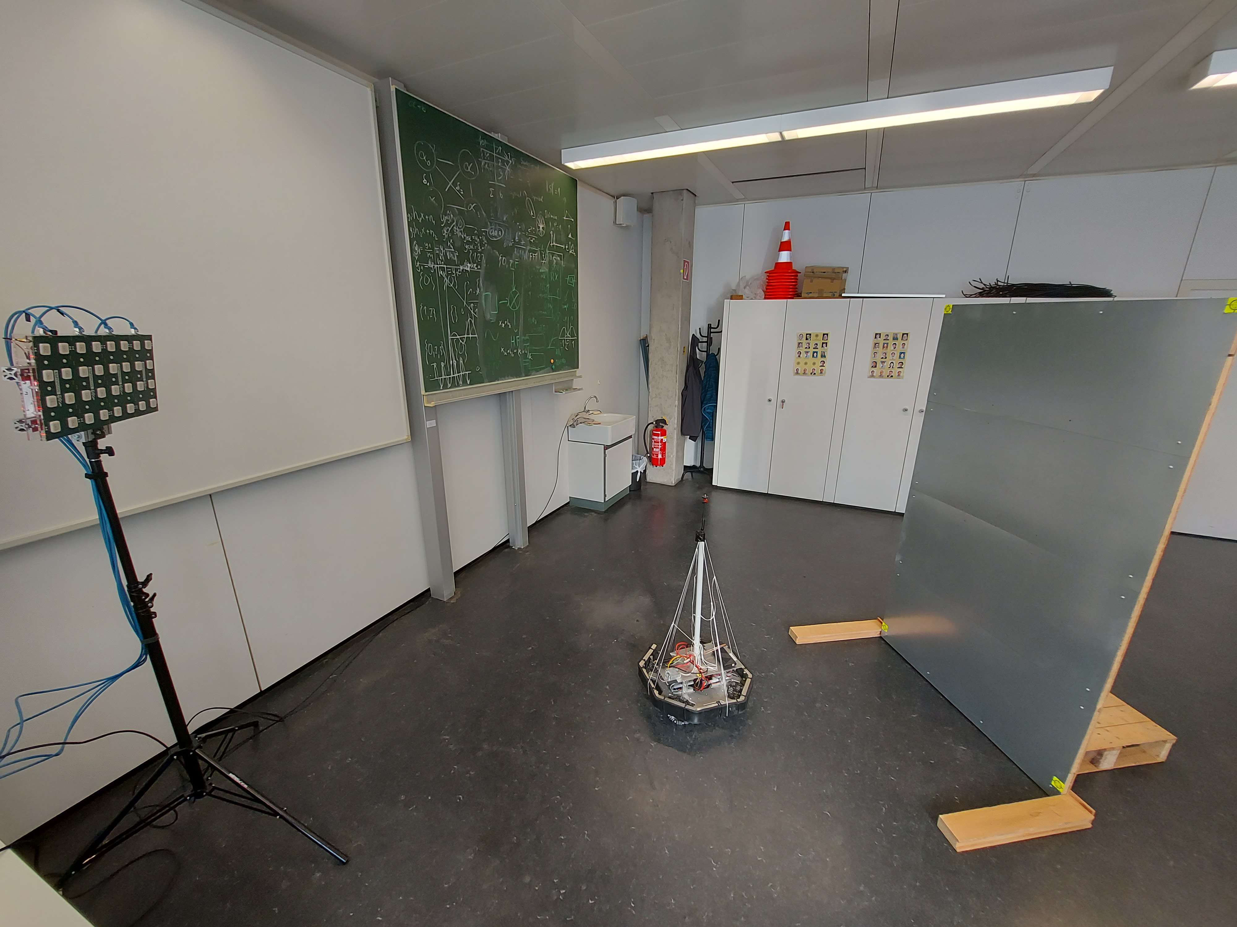
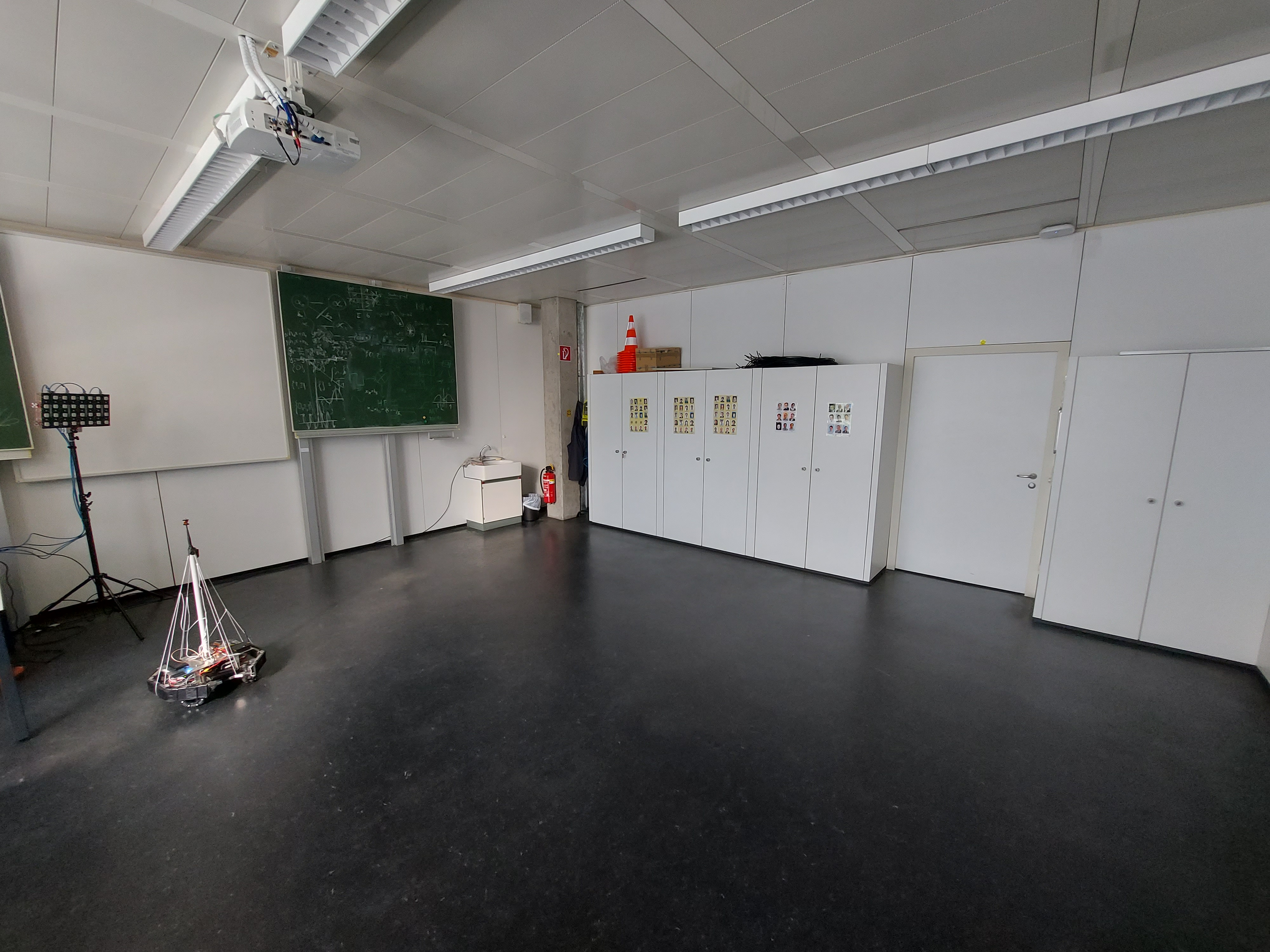
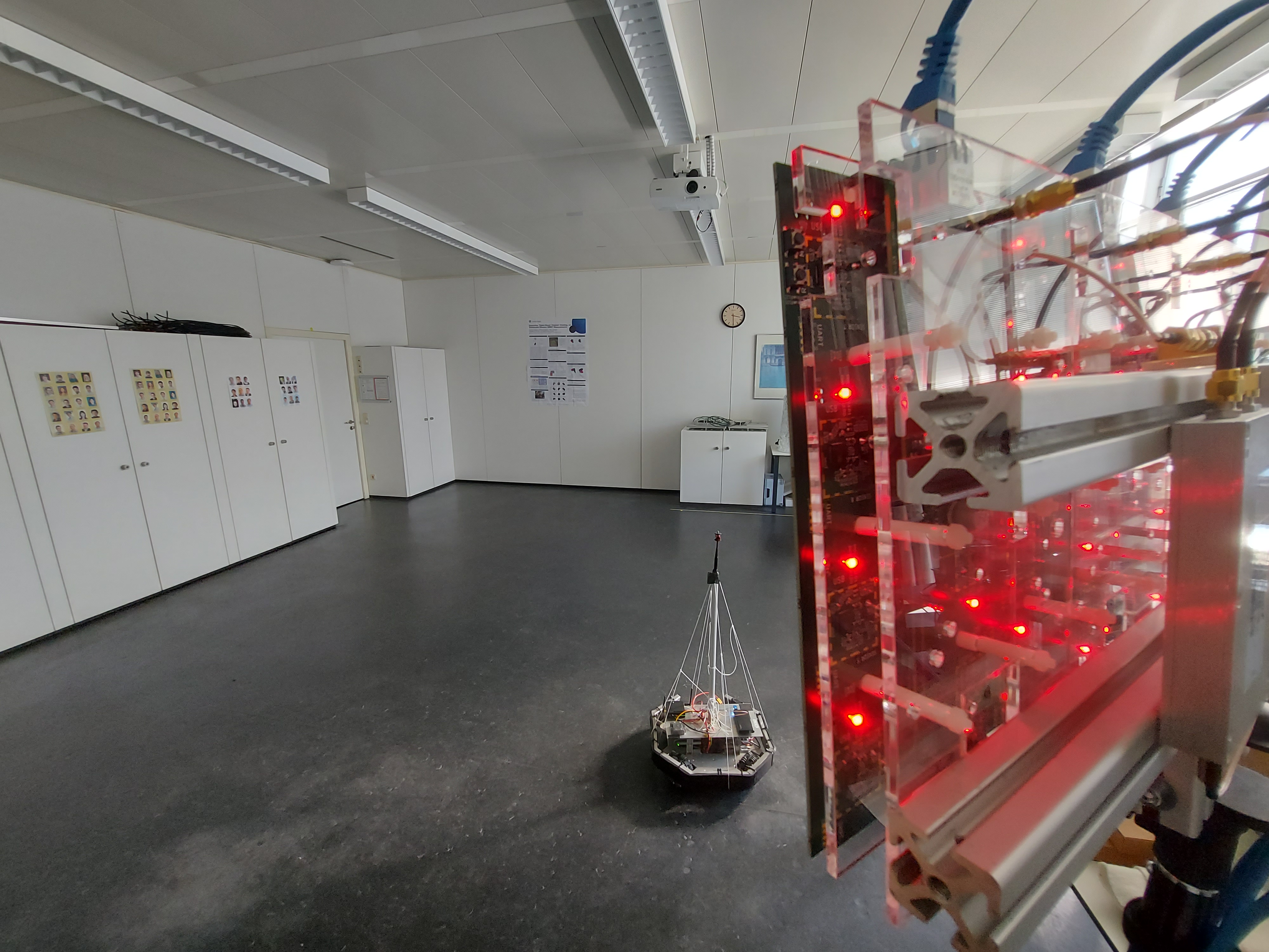
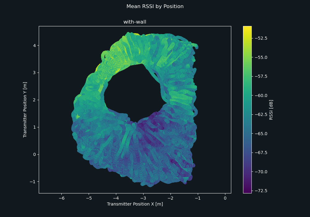
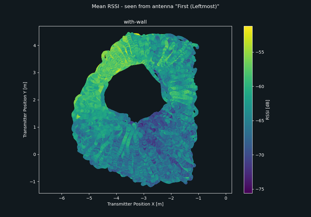
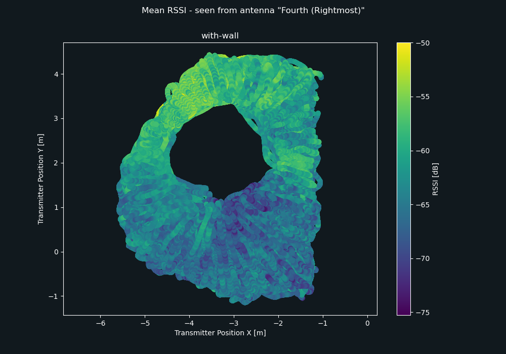
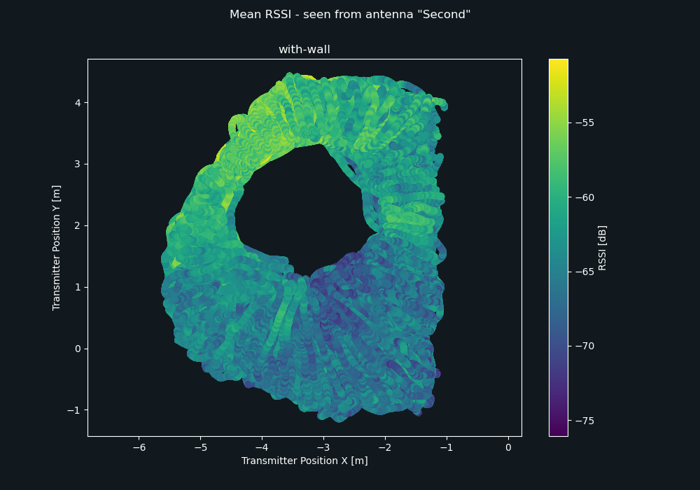
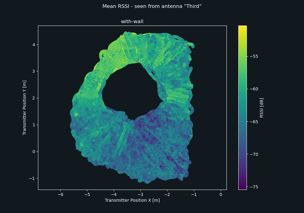
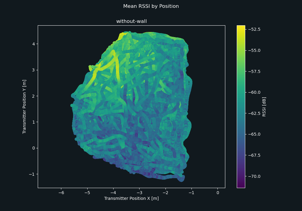
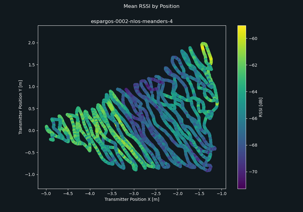
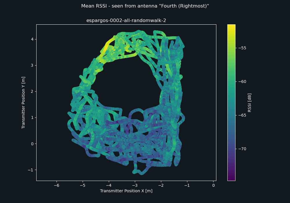
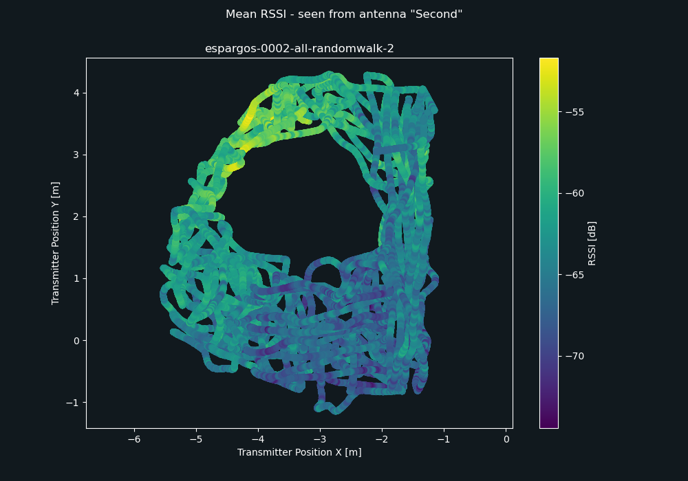
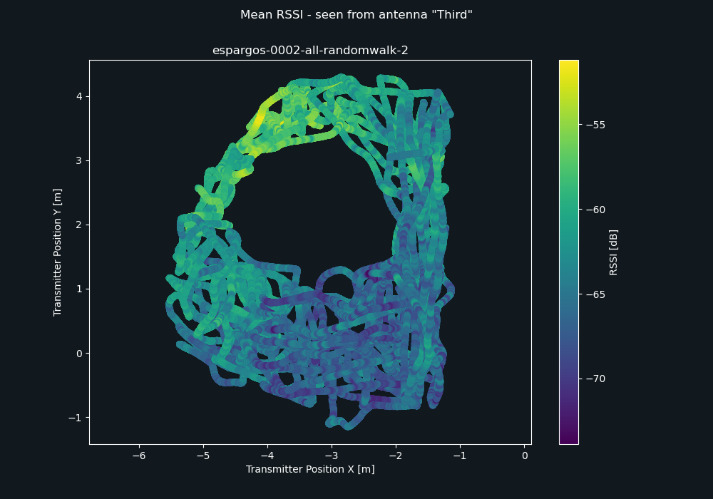
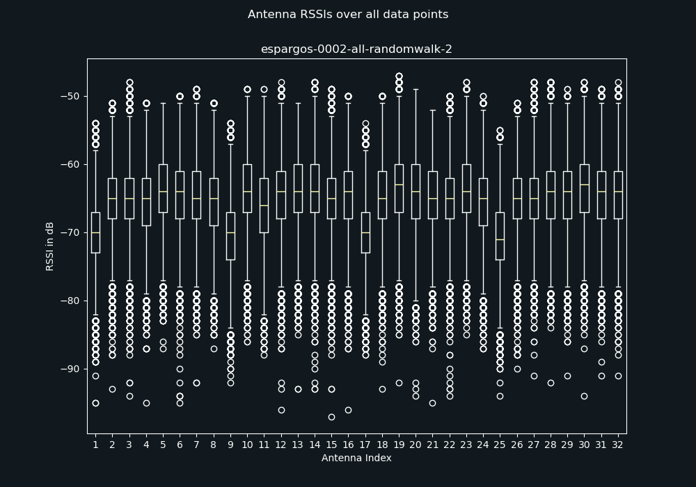
Four ESPARGOS arrays are combined into one large array with 8 by 4 antennas. A metal wall blocks the LoS path in parts of the measurement area. The wall is later removed.
36.562 MHz
Signal Bandwidth
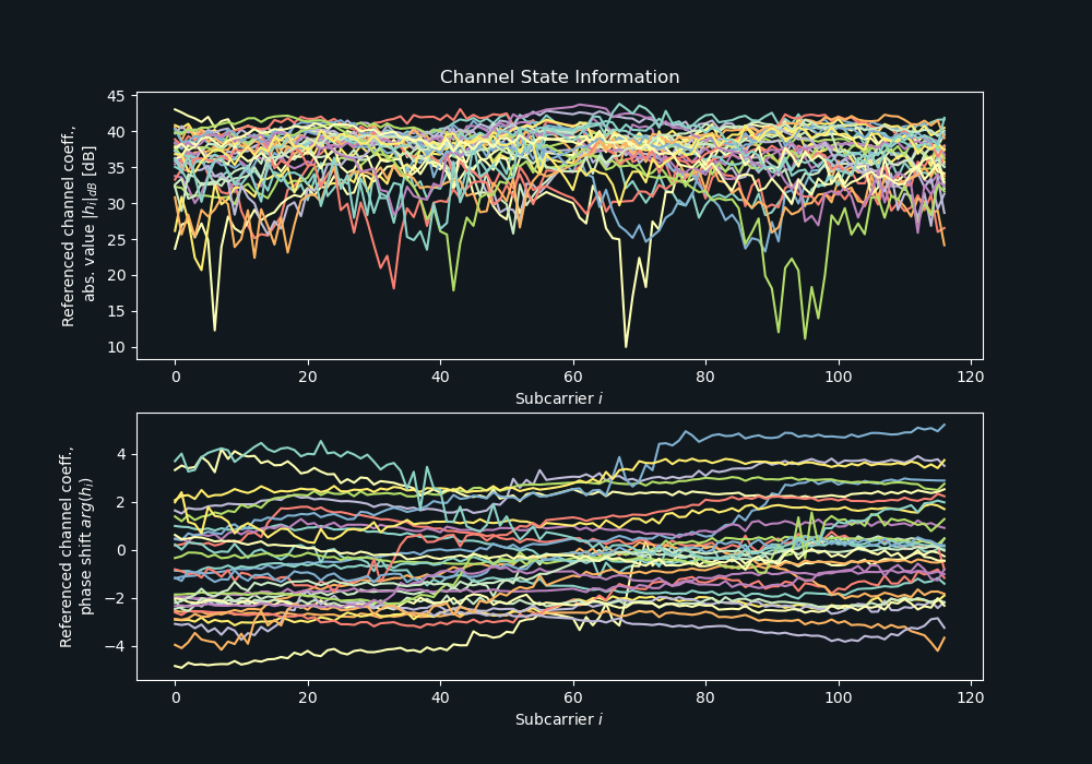
117
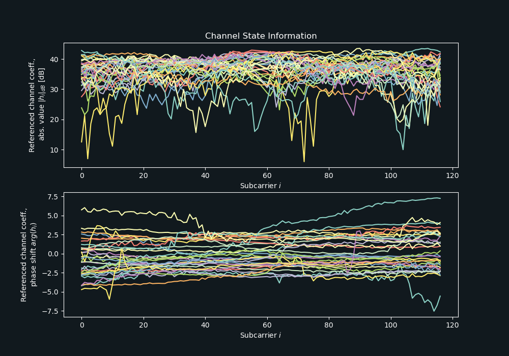
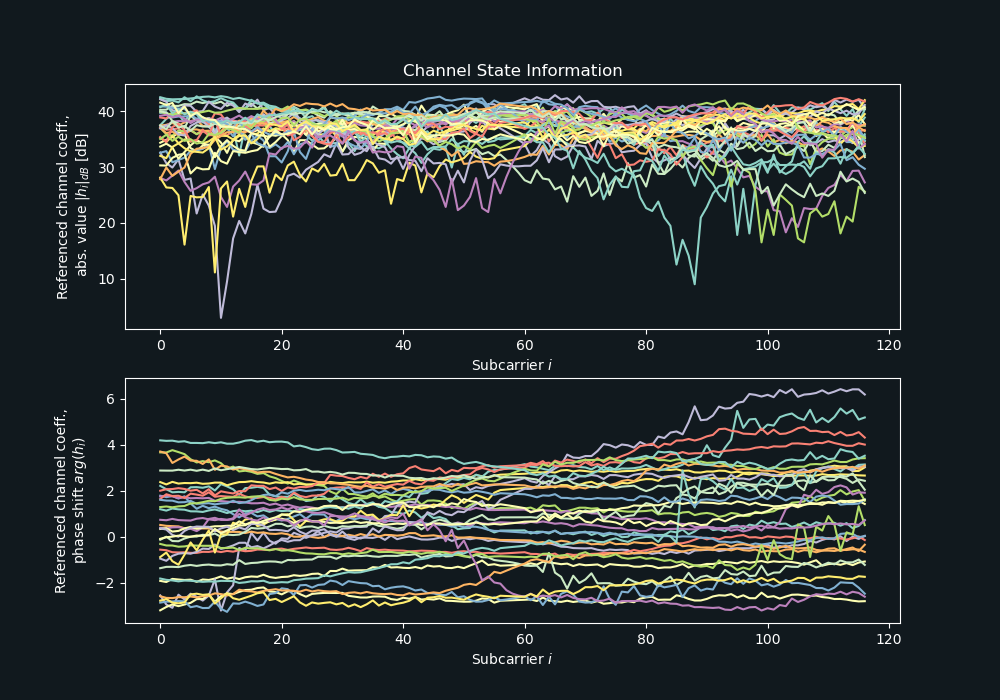
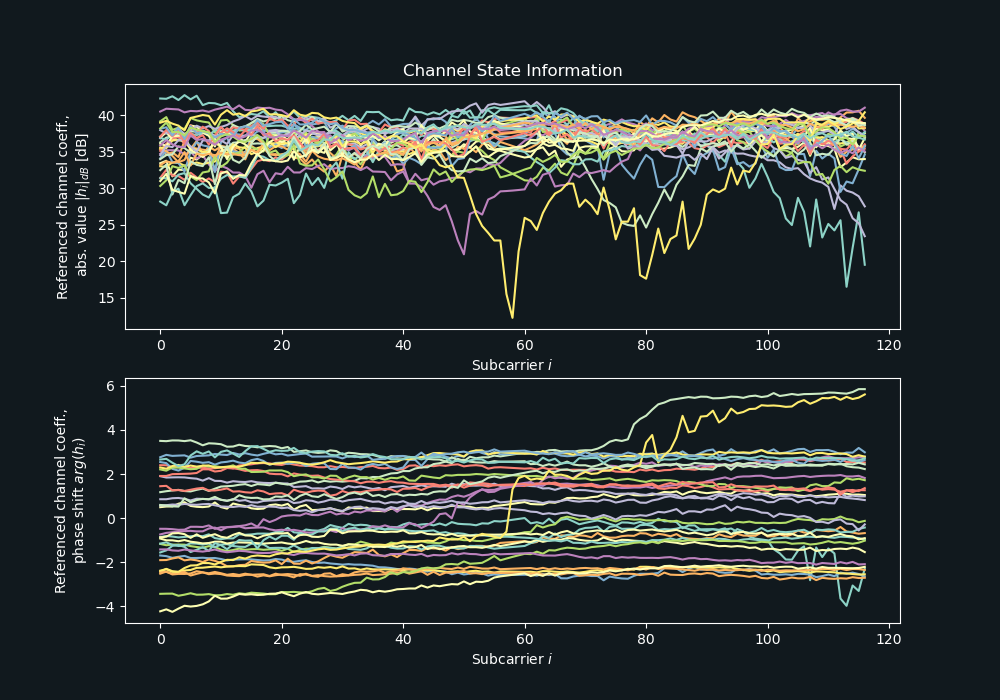
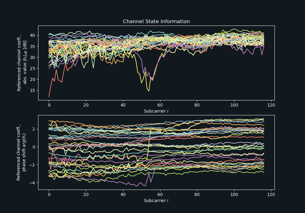
OFDM Subcarriers
2859804
Data Points
25176.2 s
Total Duration
86.5 GB
Total Download Size
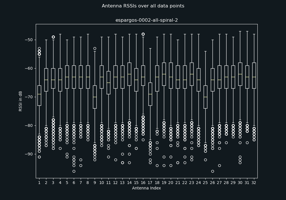
32
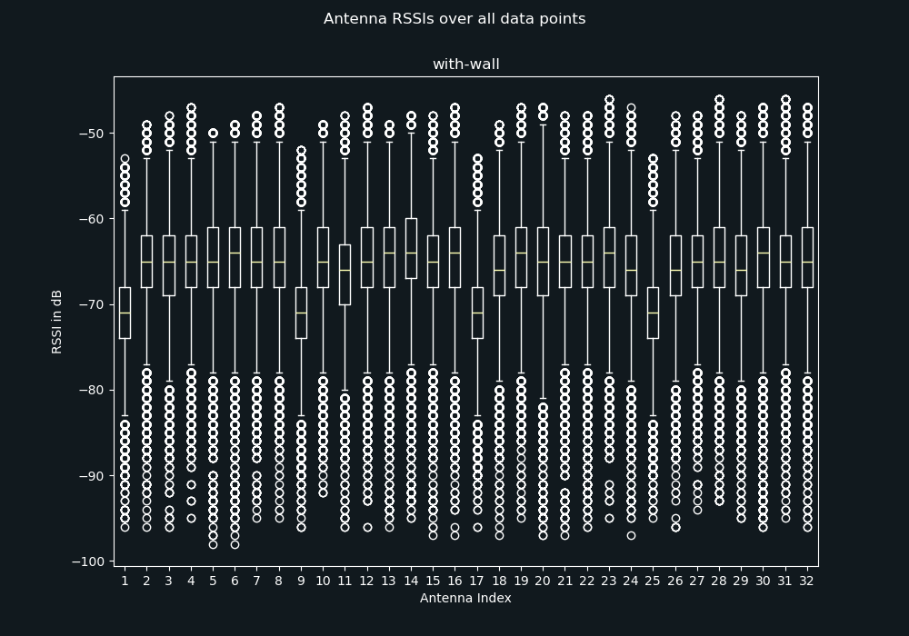
Number of Antennas
Indoor
Type of Environment
2.462000 GHz
Carrier Frequency
Global
Phase Synchronization
3D Tachymeter
Position-Tagged
802.11n
WiFi Standard
Experiment Setup
Data Analysis
Warnings
Receiver Array Setup
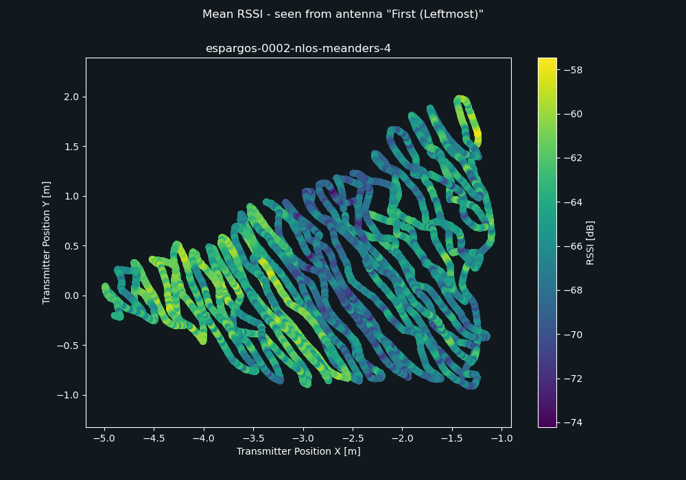
ESPARGOS 1: First (Leftmost)
ESPARGOS 2: Second
ESPARGOS 3: Third
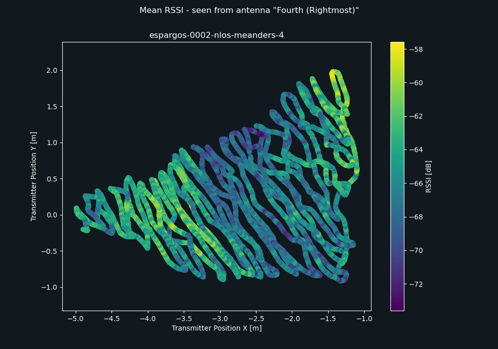
ESPARGOS 4: Fourth (Rightmost)
Python: Import with TensorFlow
#!/usr/bin/env python3
import tensorflow as tf

raw_dataset = tf.data.TFRecordDataset(["tfrecords/espargos-0002-nlos-meanders-1.tfrecords", "tfrecords/espargos-0002-nlos-meanders-2.tfrecords", "tfrecords/espargos-0002-nlos-meanders-3.tfrecords", "tfrecords/espargos-0002-nlos-meanders-4.tfrecords", "tfrecords/espargos-0002-nlos-randomwalk-1.tfrecords", "tfrecords/espargos-0002-nlos-randomwalk-2.tfrecords", "tfrecords/espargos-0002-all-spiral-1.tfrecords", "tfrecords/espargos-0002-all-spiral-2.tfrecords", "tfrecords/espargos-0002-all-randomwalk-1.tfrecords", "tfrecords/espargos-0002-all-randomwalk-2.tfrecords", "tfrecords/espargos-0002-all-randomwalk-3.tfrecords", "tfrecords/espargos-0002-all-radial-meanders-1.tfrecords", "tfrecords/espargos-0002-all-radial-meanders-2.tfrecords", "tfrecords/espargos-0002-no-wall-meanders-1.tfrecords", "tfrecords/espargos-0002-no-wall-meanders-2.tfrecords", "tfrecords/espargos-0002-no-wall-randomwalk-1.tfrecords", "tfrecords/espargos-0002-no-wall-randomwalk-2.tfrecords", "tfrecords/espargos-0002-no-wall-randomwalk-3.tfrecords"])

feature_description = {
	"csi": tf.io.FixedLenFeature([], tf.string, default_value = ''),
	"pos": tf.io.FixedLenFeature([], tf.string, default_value = ''),
	"rssi": tf.io.FixedLenFeature([], tf.string, default_value = ''),
	"time": tf.io.FixedLenFeature([], tf.string, default_value = ''),
}

def record_parse_function(proto):
	record = tf.io.parse_single_example(proto, feature_description)

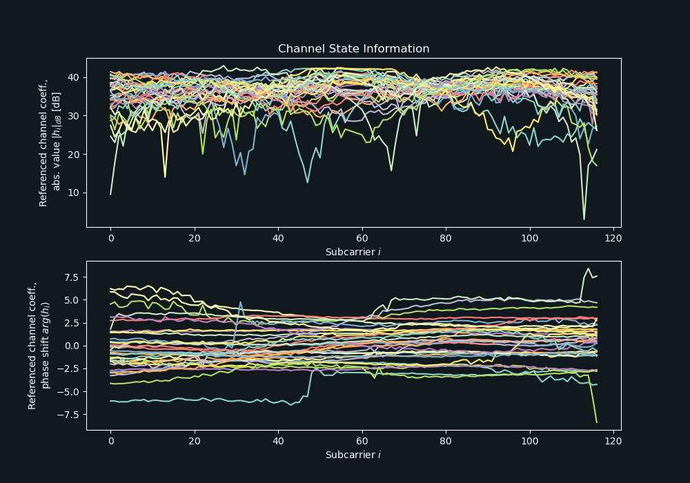
	# Channel coefficients for all antennas, over all subcarriers, complex-valued
	csi = tf.ensure_shape(tf.io.parse_tensor(record["csi"], out_type = tf.complex64), (4, 2, 4, 117))

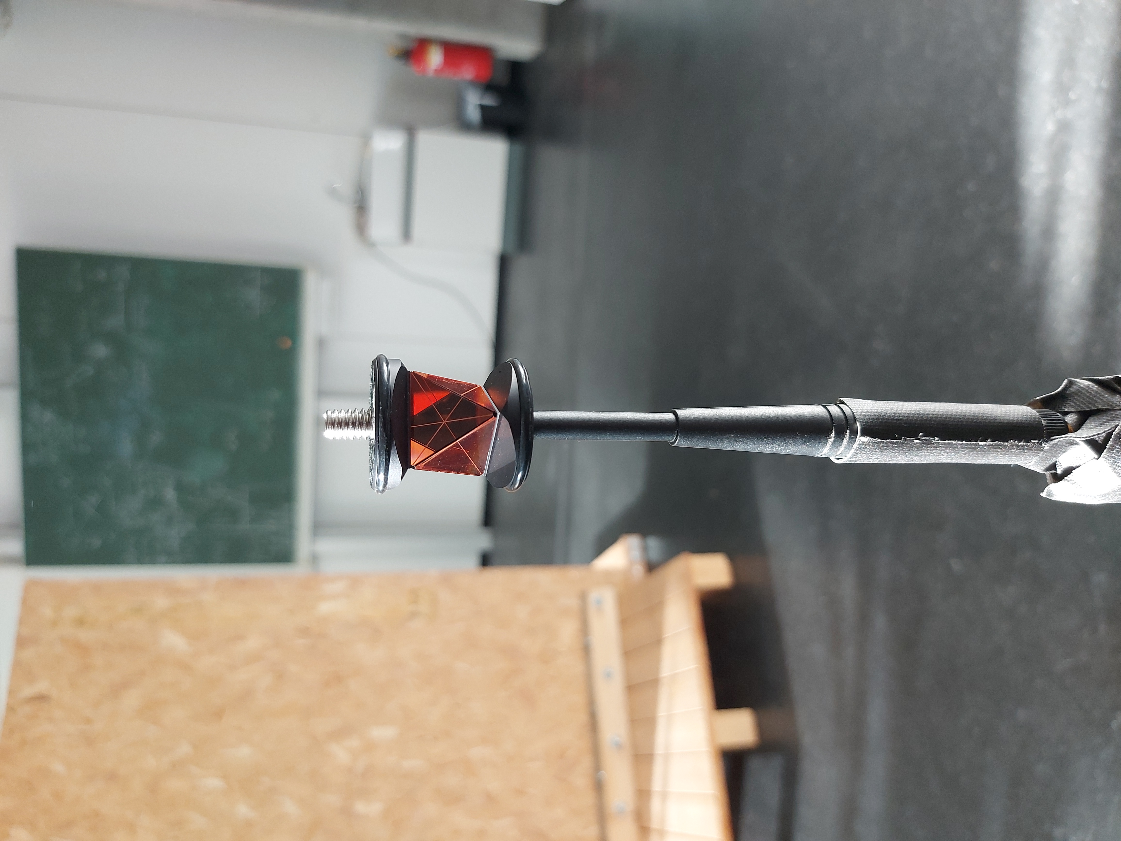
	# Position of transmitter determined by a tachymeter pointed at a prism mounted on top of the antenna, in meters (X / Y / Z coordinates)
	pos = tf.ensure_shape(tf.io.parse_tensor(record["pos"], out_type = tf.float64), (3))

	# Received signal strength indicator (in dB) for all antennas
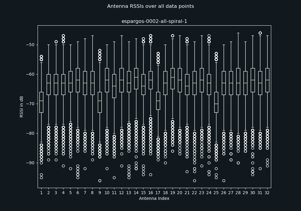
	rssi = tf.ensure_shape(tf.io.parse_tensor(record["rssi"], out_type = tf.float32), (4, 2, 4))

	# Timestamp of measurement, seconds since UNIX epoch
	time = tf.ensure_shape(tf.io.parse_tensor(record["time"], out_type = tf.float64), ())

	return csi, pos, rssi, time

dataset = raw_dataset.map(record_parse_function, num_parallel_calls = tf.data.experimental.AUTOTUNE)

# Optional: Cache dataset in RAM for faster training
dataset = dataset.cache()
Python: Combining sub-arrays into large arrays
This dataset contains 1 combined antenna array.
A combined antenna array is a large array that is made up of multiple phase-synchronized ESPARGOS arrays mounted next to each other.
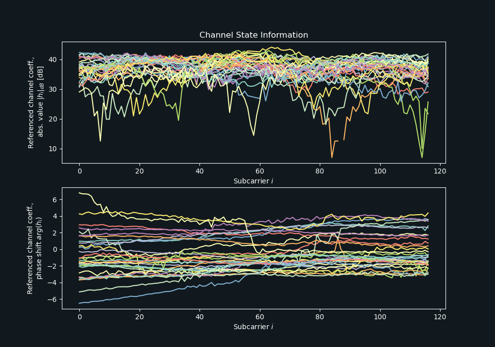
However, the csi records in the dataset files contains the channel coefficients in the usual format, i.e., in a multi-dimensional array of shape B × 2 × 4 × Nsub, where B is the number of antenna arrays and Nsub is the number of subcarriers.
You might prefer to have the CSI data of the combined antenna array in a multidimensional array of format R × M × Nsub, where R is the number of rows in the combined array and M is the number of antenna columns.
The following Python source code takes care of reshaping CSI data into that format.
assignments = [
	[(0, 1, 0), (0, 0, 0), (1, 1, 0), (1, 0, 0), (2, 1, 0), (2, 0, 0), (3, 1, 0), (3, 0, 0)],
	[(0, 1, 1), (0, 0, 1), (1, 1, 1), (1, 0, 1), (2, 1, 1), (2, 0, 1), (3, 1, 1), (3, 0, 1)],
	[(0, 1, 2), (0, 0, 2), (1, 1, 2), (1, 0, 2), (2, 1, 2), (2, 0, 2), (3, 1, 2), (3, 0, 2)],
	[(0, 1, 3), (0, 0, 3), (1, 1, 3), (1, 0, 3), (2, 1, 3), (2, 0, 3), (3, 1, 3), (3, 0, 3)]
]

dataset = dataset.map(lambda csi, rssi, *args : (tf.gather_nd(csi, assignments), tf.gather_nd(rssi, assignments), *args))
Configuration Variants and Pointcloud
:
Pointcloud Download and Usage Instructions
For this dataset, we provide a pointcloud of the environment, which was generated using a 3D scanning device. You may find the pointcloud useful for visualization purposes or to reconstruct and verify 3D models. Pointclouds can be viewed and edited with applications like CloudCompare.
The tachymeter was used to create multiple pointcloud scans. During the measurement campaign, i.e., while the robot was moving, the tachymeter was stationed outside of the measurement area, but was moved there for making the pointcloud scan. The coordinate system of the pointlcoud is the same coordinate system that was also used for the rest of the dataset (datapoint positions, antenna array positions). We achieve this using some reference position markers in the room. Due to small errors in the measurement of these reference positions, there might also be small errors in the pointcloud coordinates.
The pointclouds are available for download as .pts files inside a .tar.xz archive.
The following pointcloud scans are available:
with-wall-wood.pts: Pointcloud for configuration variant with metal wall. The tachymeter was stationed on the “wooden” site of the wall, i.e., between metal wall and antenna array.with-wall-metal.pts: Pointcloud for configuration variant with metal wall. The tachymeter was stationed on the “metallic” site of the wall, i.e., between metal wall and lab room door.no-wall.pts: Pointcloud for configuration variant without metal wall
PTS files are simple text files with the following format:
- The first line contains the number of datapoints in the scan
- The other lines contain
(x, y, z)coordinates, reflection intensity and(r, g, b)color, e.g.:
x      y        z       i    r   g   b
6.9912 -19.5173 14.7111 -546 183 190 174
6.9930 -19.5178 14.7112 -505 162 171 154
6.9888 -19.5181 14.7098 -570 193 200 184
6.9902 -19.5111 14.7109 -578 184 191 173
How to Cite
Please refer to the home page for information on how to cite any of our datasets in your research. For this dataset in particular, you may use the following BibTeX:
@data{dataset-espargos-0002,
	author    = {Euchner, Florian and ten Brink, Stephan},
	publisher = {DaRUS},
	title     = {{CSI Dataset espargos-0002: Larger combined antenna array, indoor lab room with metal wall, LoS and NLoS areas}},
	doi       = {doi:10.18419/darus-4456},
	url       = {https://doi.org/doi:10.18419/darus-4456},
	year      = {2024}
}
A Note on WiFi Subcarriers, Bandwidth and Interpolation
WiFi has a concept of "guard" subcarriers, which act as guard bands that protect against interference with systems on neighboring WiFi channels. This means that not all subcarriers get driven (i.e., not all subcarriers contain useful QAM symbols), some subcarriers simply carry zeroes. If these subcarriers are at the edge of the considered spectrum, CSI from these guard subcarriers is simply not included in the dataset. This explains the odd (non-power of two) number of subcarriers. Therefore, even if we colloquially refer to WiFi bandwidths as "20MHz" or "40MHz", the bandwidth that is really occupied by the active OFDM subcarriers is lower. For "missing" subcarriers in the center of the bandwidth (DC subcarrier in the case of 20MHz bandwidth, guard subcarriers in the case of 40MHz bandwidth), linear interpolation is used to assign realistic values to them.
A Note on Synchronization
To make sense of the measured CSI data, please take into account:- Lack of time synchronization: While ESPARGOS ensures phase synchronization across antennas in the same array, due to an esp-idf software limitation at the time of creating this dataset, there is no sampling time synchronization.
Download
This dataset consists of 18 files. Descriptions of these files as well as download links are provided below.
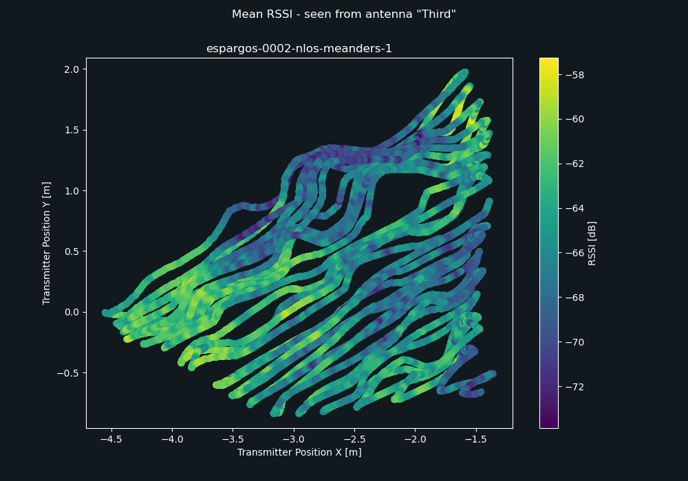
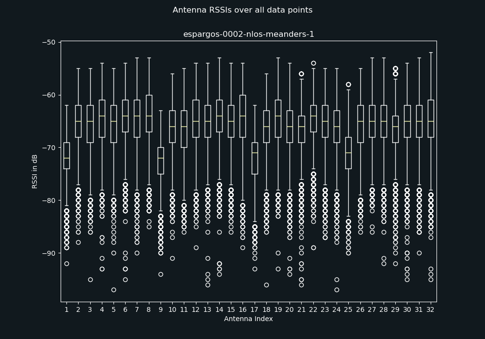
espargos-0002-nlos-meanders-1
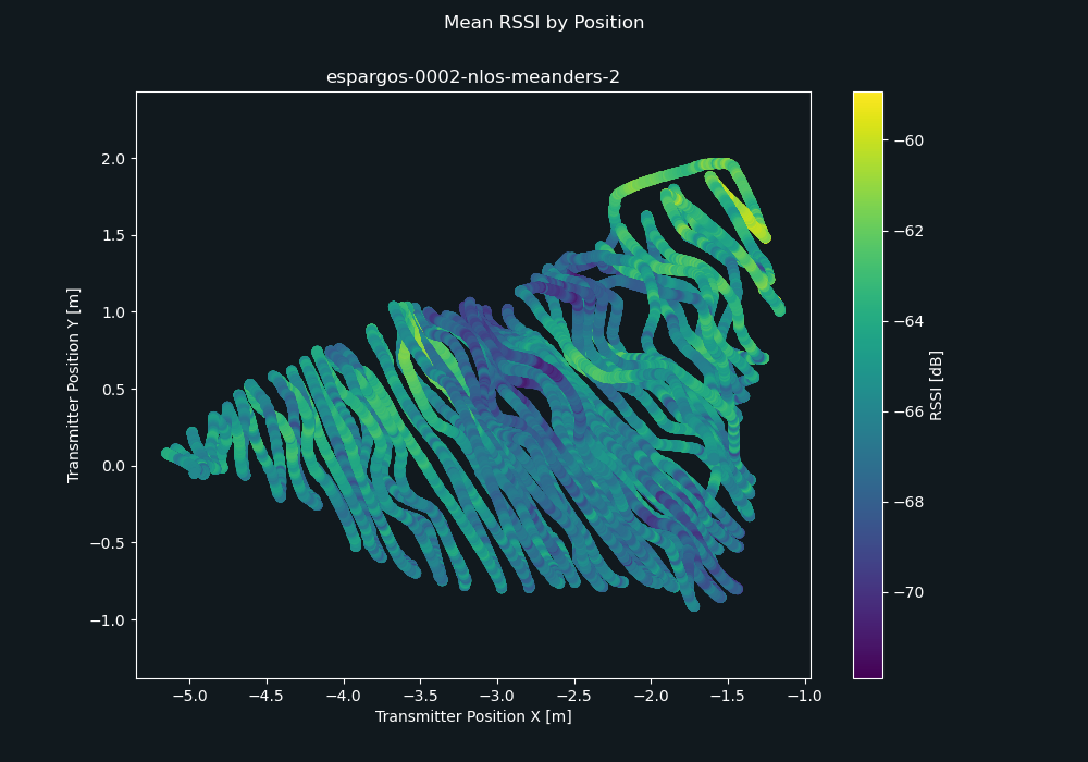
espargos-0002-nlos-meanders-2
espargos-0002-nlos-meanders-3
espargos-0002-nlos-meanders-4
espargos-0002-nlos-randomwalk-1
espargos-0002-nlos-randomwalk-2
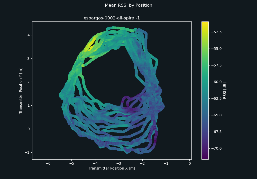
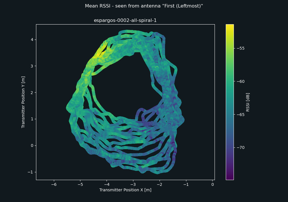
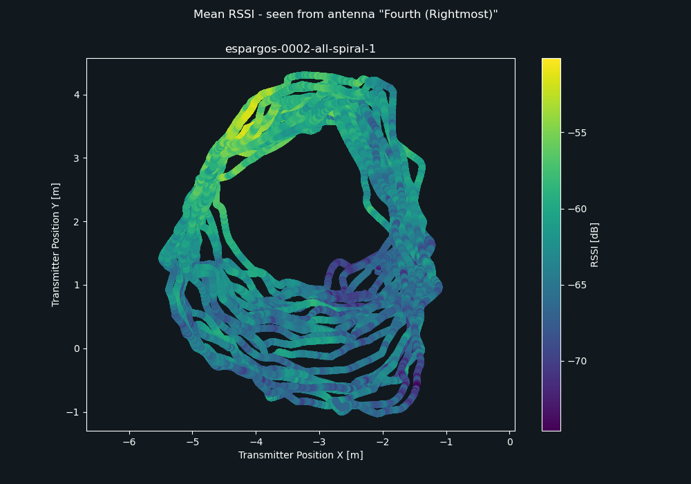
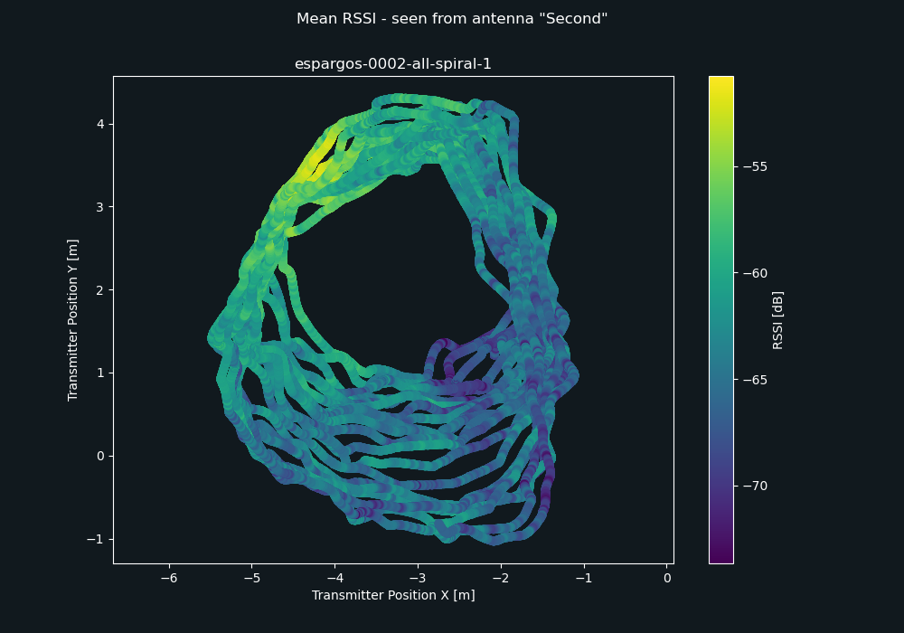
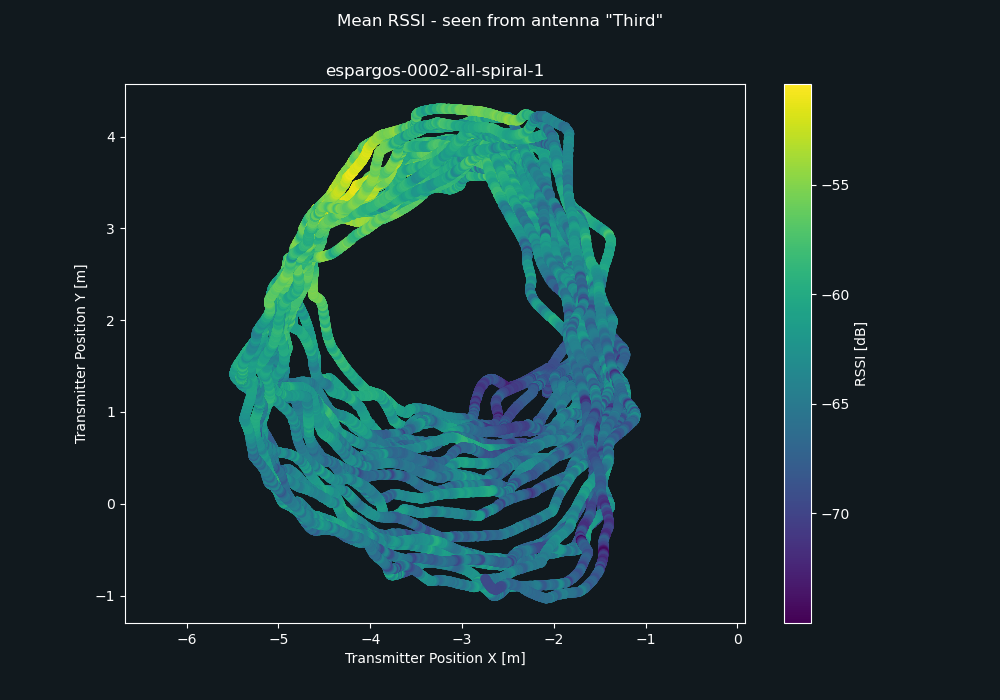
espargos-0002-all-spiral-1
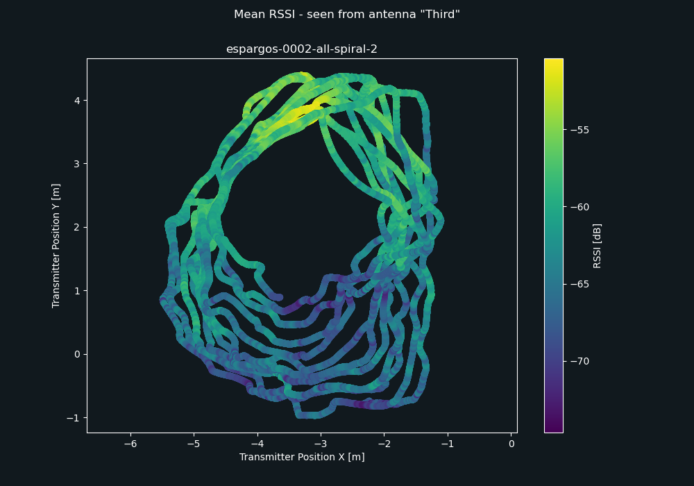
Robot follows a trajectory of clockwise spirals (when viewed from top) around the metal wall, travelling through LoS and NLoS areas of the measurement area.
File Size
Data Points
Duration
espargos-0002-all-spiral-2
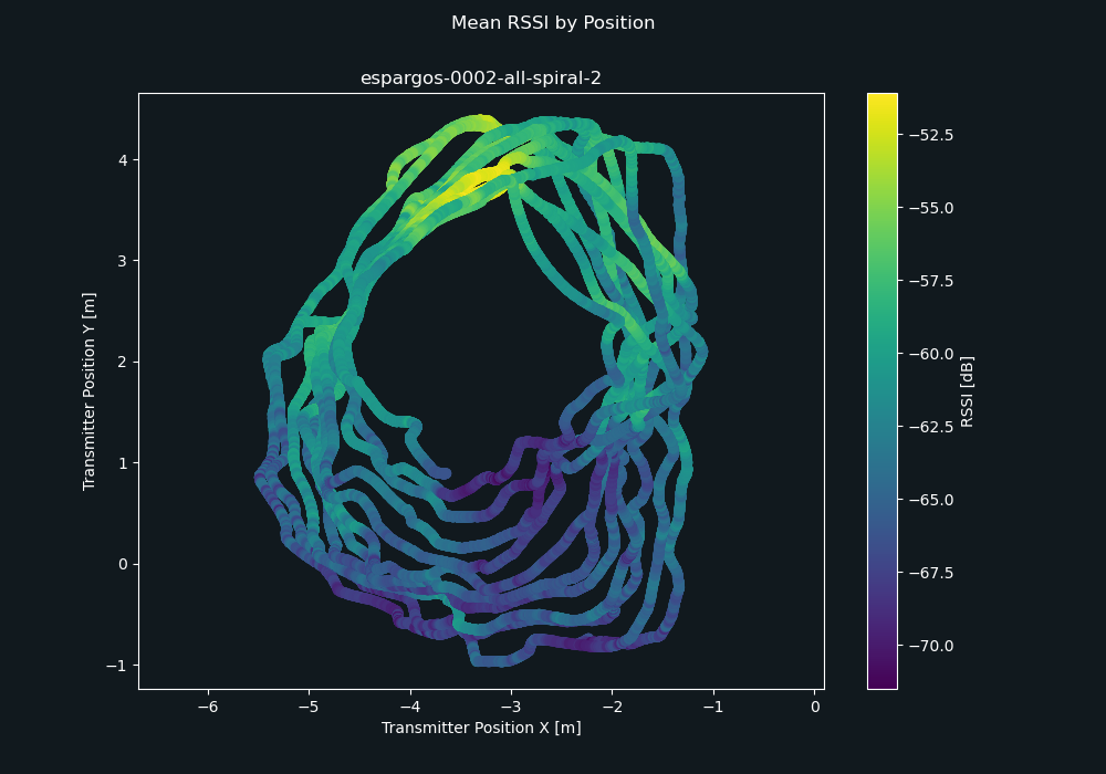
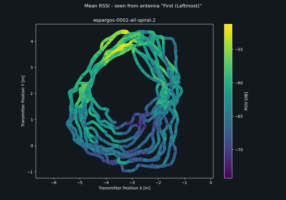
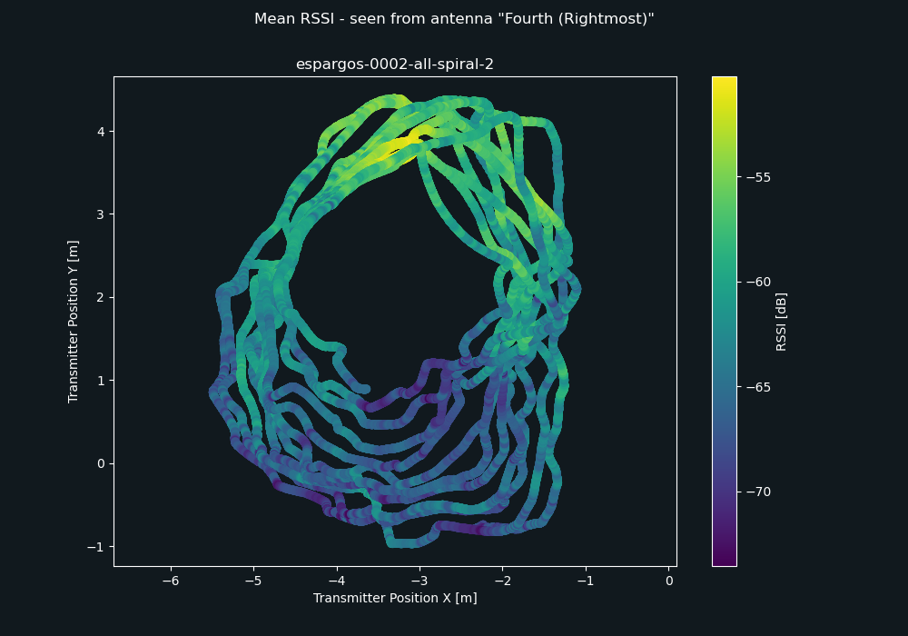
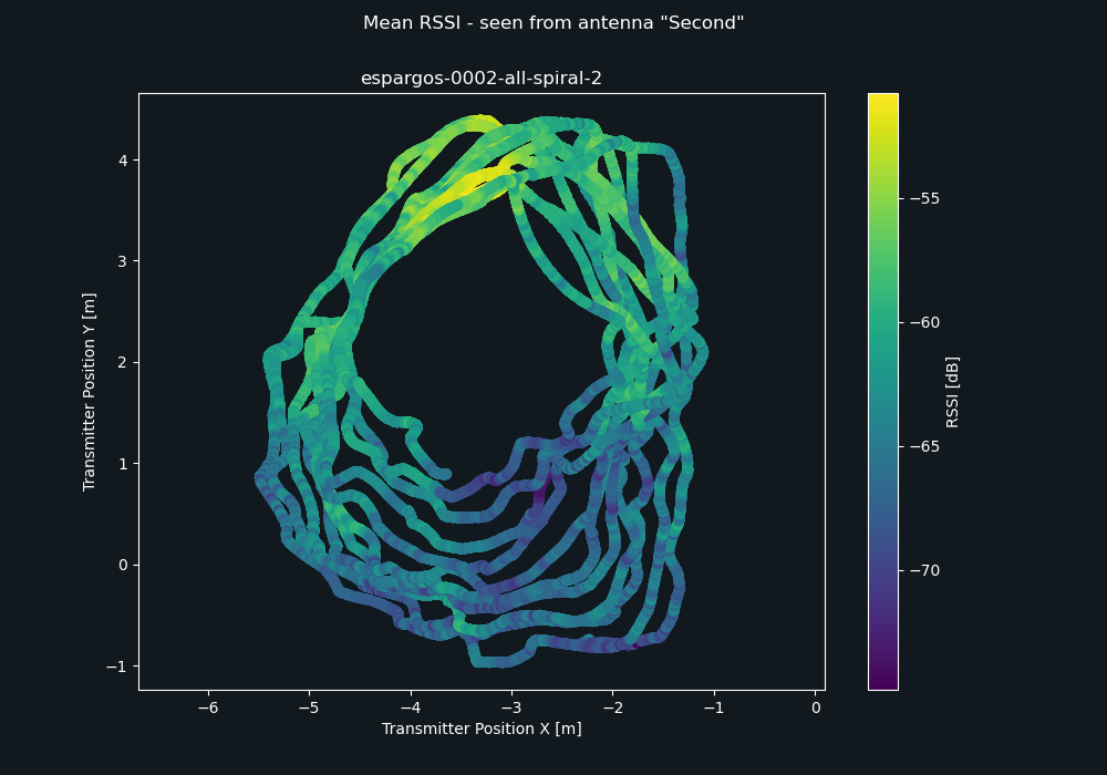
Robot follows a trajectory of counter-clockwise spirals (when viewed from top) around the metal wall, travelling through LoS and NLoS areas of the measurement area.
File Size
Data Points
Duration
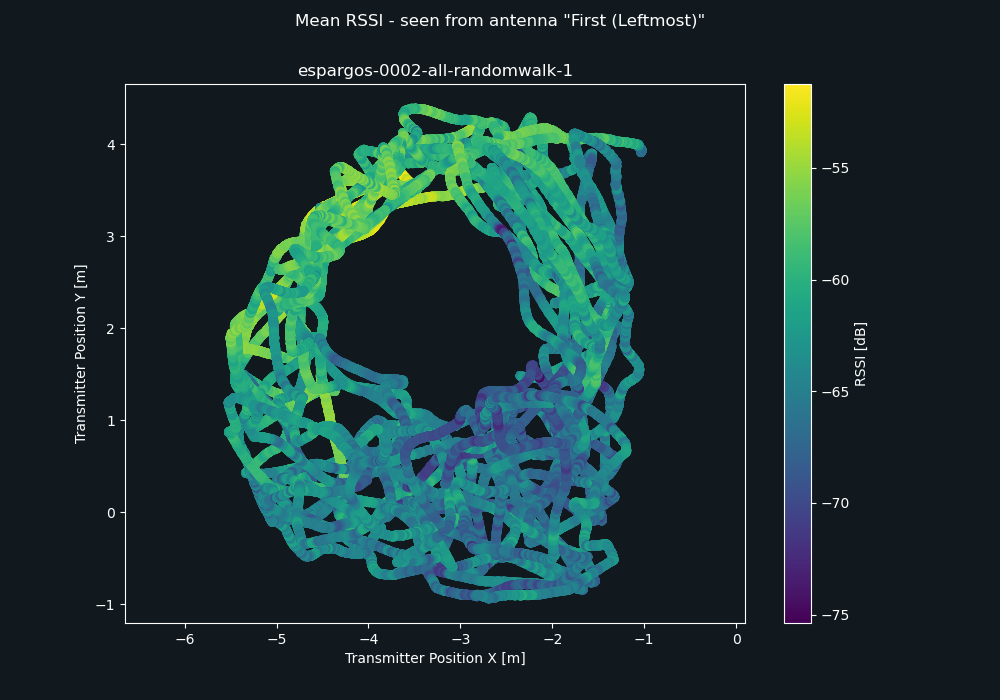
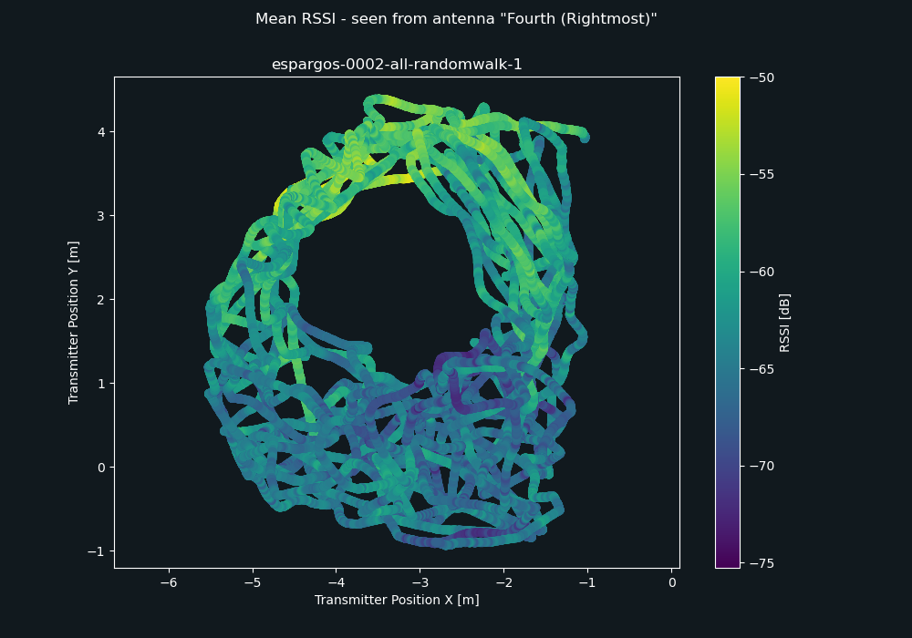
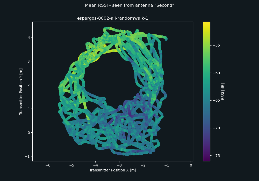
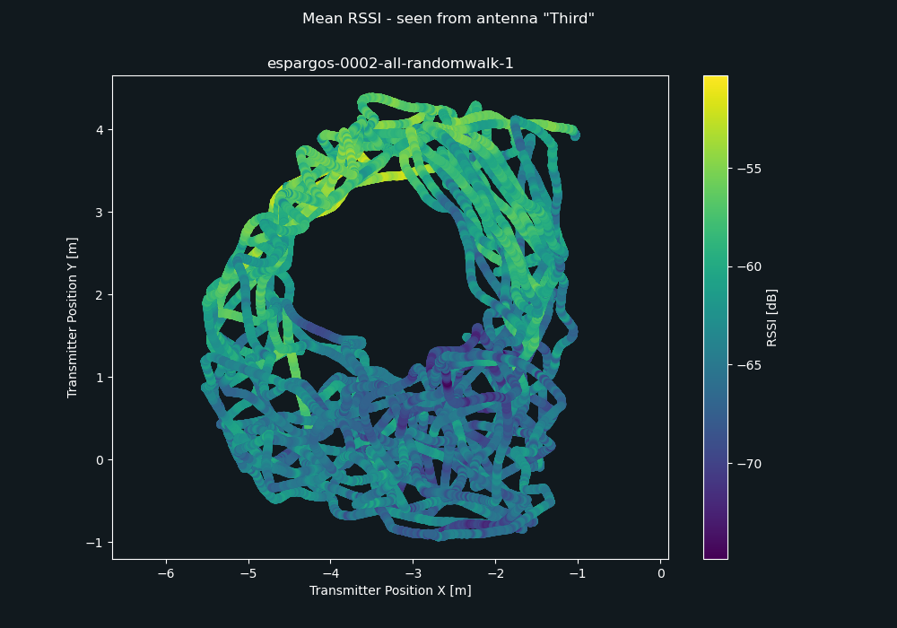
espargos-0002-all-randomwalk-1
espargos-0002-all-randomwalk-2
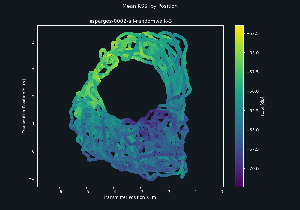
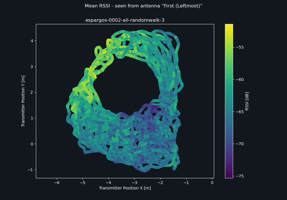
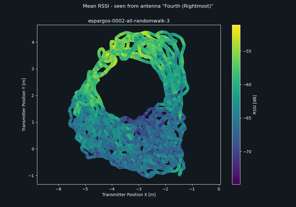
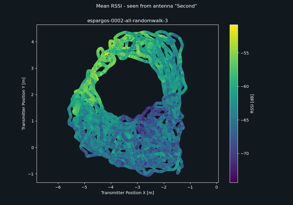
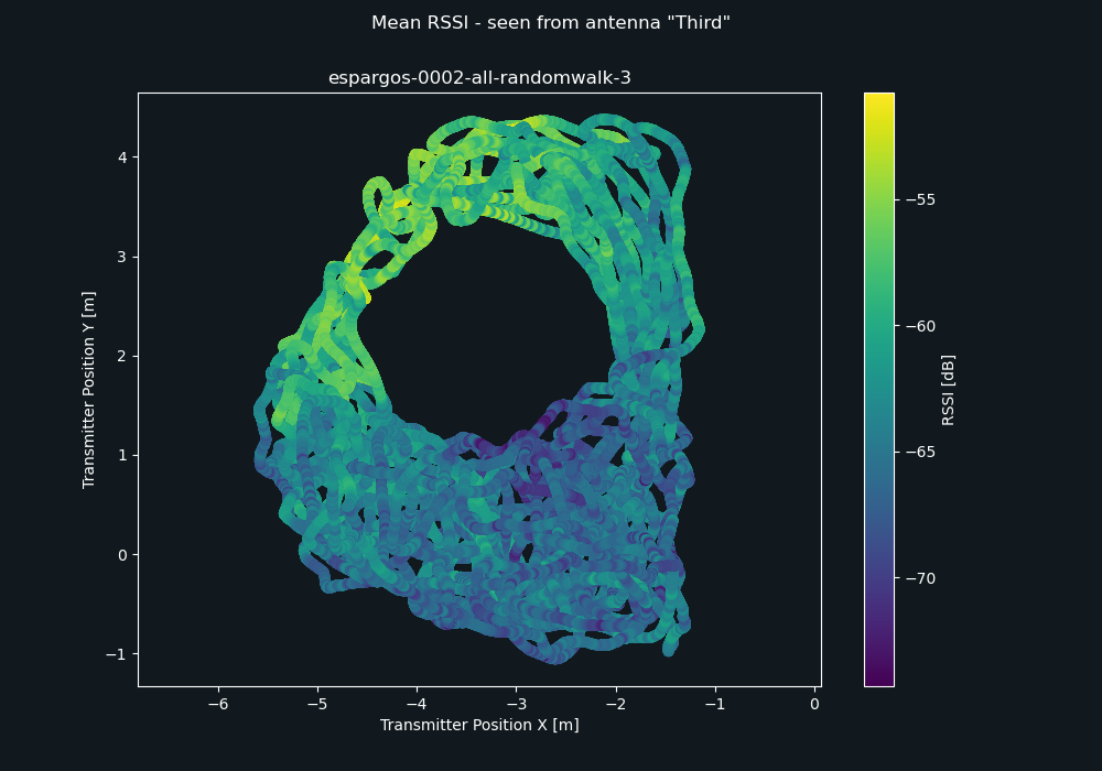
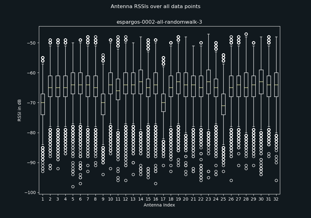
espargos-0002-all-randomwalk-3
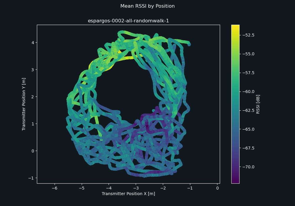
Robot follows a pseudorandom trajectory all around the metal wall, containing both LoS and NLoS areas. Robot movement is slower than all-randomwalk-1 and all-randomwalk-2.
File Size
Data Points
Duration
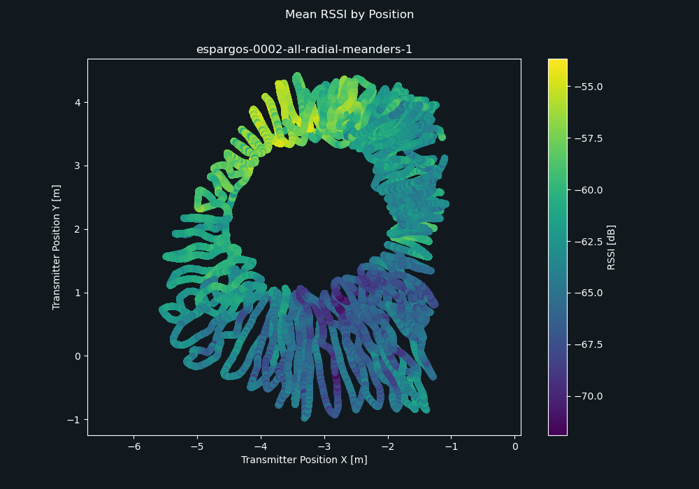
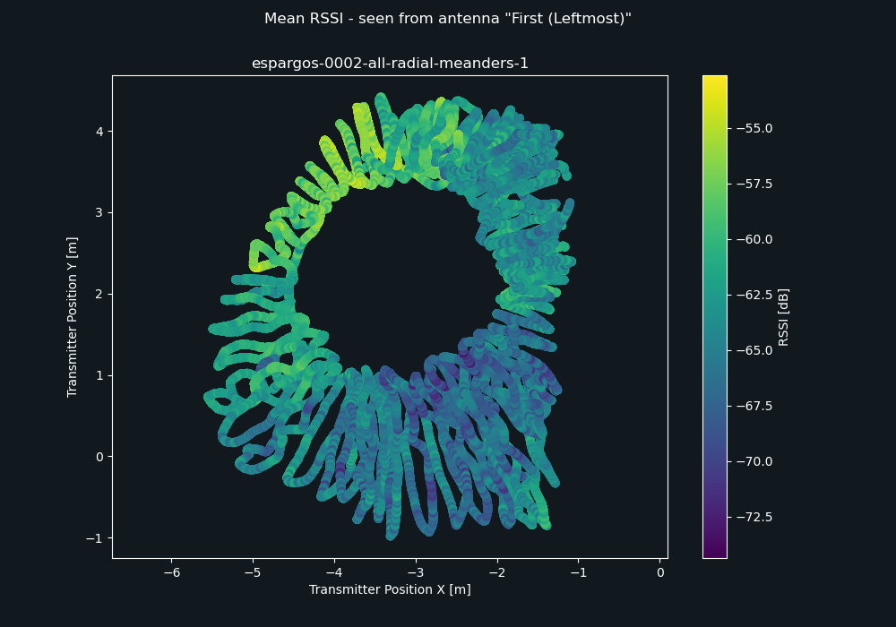
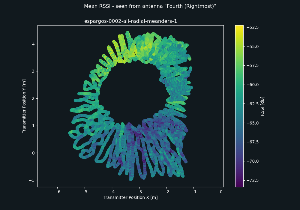
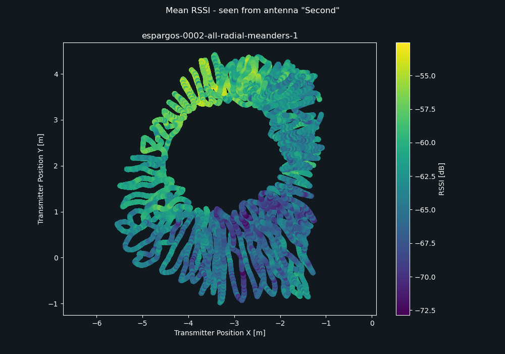
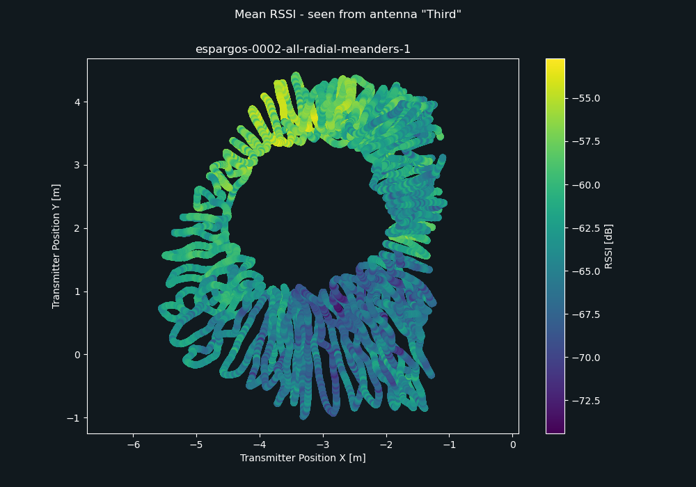
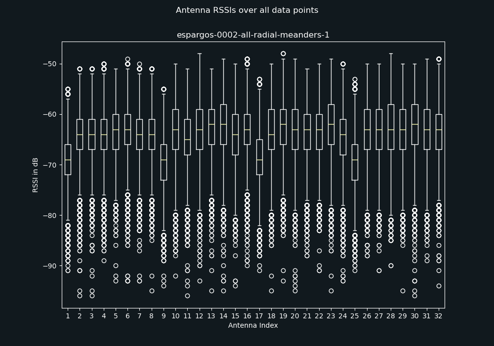
espargos-0002-all-radial-meanders-1
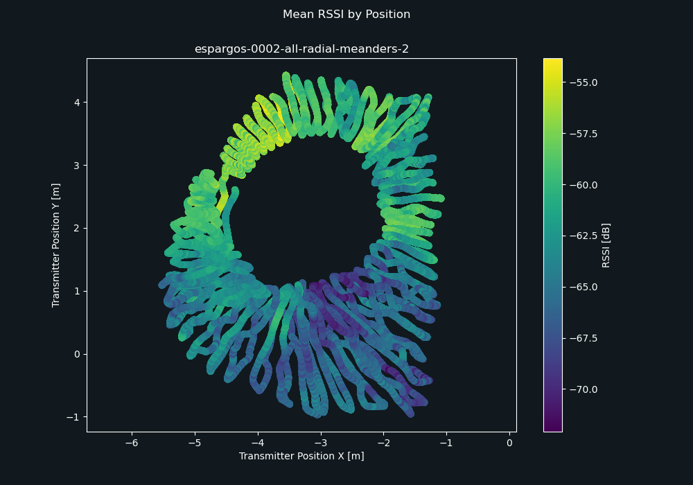
espargos-0002-all-radial-meanders-2
espargos-0002-no-wall-meanders-1
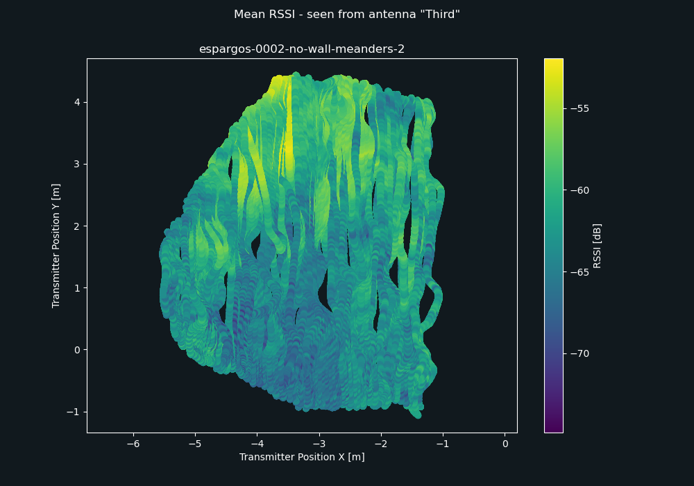
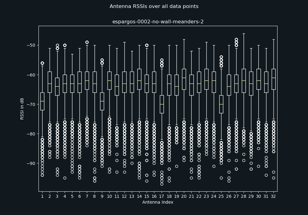
espargos-0002-no-wall-meanders-2
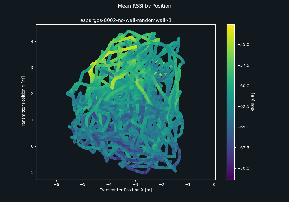
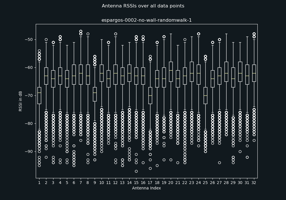
espargos-0002-no-wall-randomwalk-1
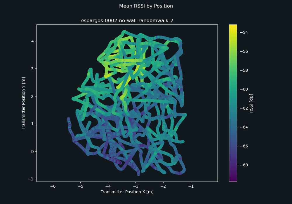
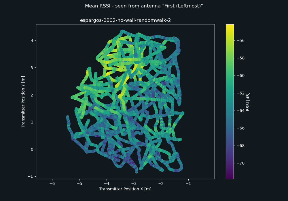
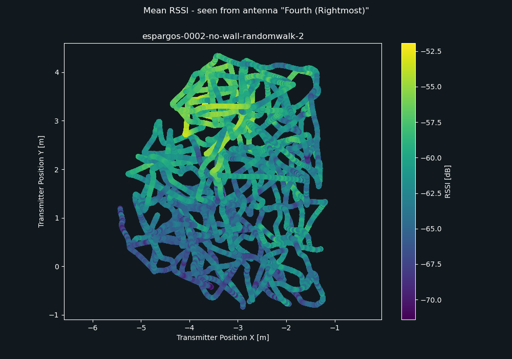
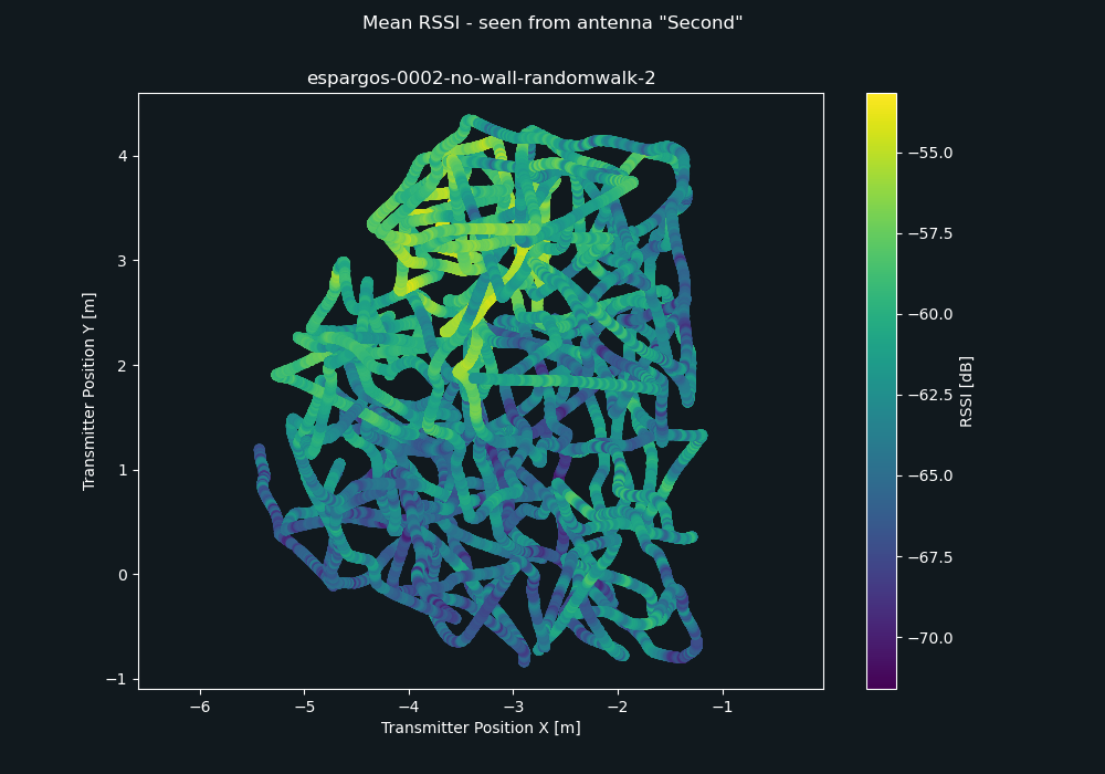
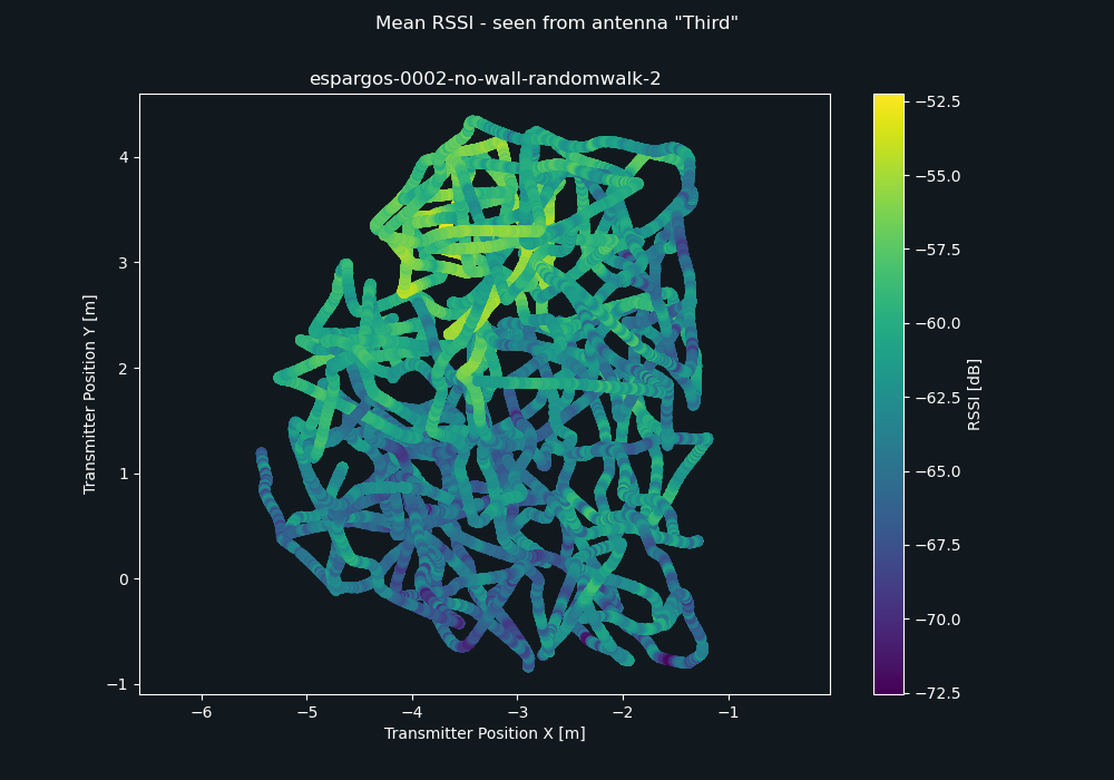
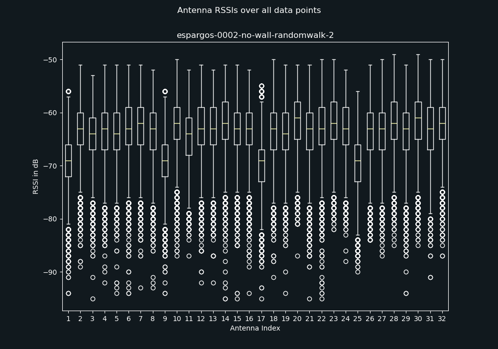
espargos-0002-no-wall-randomwalk-2
